Kinematics and Projectile Motion

Source: Ketron Mitchell-Wynne, PhD, Asantha Cooray, PhD, Department of Physics & Astronomy, School of Physical Sciences, University of California, Irvine, CA

This experiment demonstrates the kinematics of motion in 1 and 2 dimensions. This lab will begin by studying motion in 1 dimension, under constant acceleration, by launching a projectile directly upward and measuring the maximum height reached. This lab will verify that the maximum height reached is consistent with the kinematic equations derived below.

Motion in 2 dimensions will be demonstrated by launching the ball at an angle θ. Using the kinematic equations below, one can predict the distance to where the projectile will land based upon the initial speed, total time, and angle of trajectory. This will demonstrate kinematic motion with and with out acceleration in the y- and x-directions, respectively.

Any measurement of the kinematics of an object, such as position, displacement, and speed, must be made with respect to some reference frame. The x-direction of the coordinate axes will correspond to the horizontal direction, and y to the vertical. The origin of the coordinate axes (0, 0), will be defined as the initial position of the particle (here, a ball).

Motion in 1 dimension

Let's begin by considering the 1-dimensional motion of a ball over some particular time interval t, corresponding to position y. Denote the initial time as t₀, which corresponds to position y₀. The displacement of the ball, Δy, is defined as:

Δy = y - y₀. (Equation 1)

The average velocity of the ball, v^-, is the displacement divided by the elapsed time:

v^-= (y - y₀)/(t - t₀) = Δx/Δt.(Equation 2)

The instantaneous velocity, v, is the velocity over some very small time interval, defined as:

v = lim_{Δt→→ 0} (Δx/Δt). (Equation 3)

The constant acceleration, a, is the change in velocity divided by the elapsed time:

a = (v - v₀)/(t - t₀). (Equation 4)

Set t₀ = 0 to be the initial time and solve for v in the last equation to obtain the velocity as a function of time:

v = v₀ + at.(Equation 5)

Next, calculate the position y as a function of time using Equation 2. y is re-labelled as:

y = y₀ + v^-t. (Equation 6)

Under constant acceleration, the velocity will increase at uniform rate, so the average velocity will be halfway between the initial and final velocities:

v^- = (v₀ + v)/2. (Equation 7)

Substituting this into Equation 6 and using the definition of instantaneous velocity gives a new equation for y:

y = y₀ + v₀t + ½ at².(Equation 8)

t is solved for by substituting Equation 7 into Equation 6:

t = (v - v₀)/a. (Equation 9)

Substituting that t into Equation 6 and again using the definition of Equation 7 again changes the equation for y:

y = y₀ + (v + v₀)/2 (v - v₀)/a = y₀ + (v^{2 -} v₀²)/2a. (Equation 10)

Solving for v² gives:

v² = v₀² + 2a(y - y₀). (Equation 11)

These are the useful equations relating position, velocity, acceleration, and time when a is constant.

Motion in 2 dimensions

Now, motion in 2 dimensions will be considered. Equations 5, 7, 8,and 11 constitute a general set of kinematic equations in the y-direction. These can be expanded to motion in 2 dimensions, x and y, by simply replacing the y components with x components. Consider a projectile launched with an initial velocity v₀at an angle θ with respect to the x-axis, as shown in Figure 1. From the figure, one can see that the x-direction component for the initial velocity, v_x,0, is v₀cos(θ). Similarly, in the y-direction, v_y,0 = v₀sin(θ).

The only acceleration the particle experiences is gravity in the negative y-direction. Therefore, the velocity in the x-direction is constant. The velocity in the y-direction reaches a minimum at the peak of the parabola, halfway through the displacement, at t/2, where t is the total time. Use the equations above to describe this 2-dimensional motion with equations. In this coordinate frame, the origin (0,0) corresponds to (x₀, y₀). Starting with the x-direction

x = x₀ + v_x,0 t + ½ a_xt² (Equation 12)

= v₀ cos(θ)t. (Equation 13)

In the y-direction

^{y = y}₀ + v_y,0t + ½ a_y t² (Equation 14)

^{= v}₀sin(θ)t - ½ g t²,(Equation 15)

Figure 1. Projectile motion in 2 dimensions. A projectile is launched with initial velocity v₀at an angle θ with respect to the x-axis. The two velocity components are v_xand v_y, where V = v_x +v_y.

where g is the gravitational acceleration. If one measures the time it takes for the projectile to complete its path and the angle θ and the initial velocity v₀ are known, the displacement in the x- and y-directions can be calculated. Before beginning this experiment, the muzzle velocity of the launcher, 6.3 m/s, is known.These displacement calculations will be compared to the experimental results. A similar procedure can be done in 1 dimension by shooting the projectile directly upwards, with θ = 0.

1. Motion in 1 dimension.

1. Obtain a ball, a launcher with a plunger, two poles, a bucket, two clamps, a bungee cord, and a 2-m stick.
2. Attach the launcher to a pole, with a 2-m length of pole above it.
3. Use the plunger to place the ball in the launcher at maximum spring tension.
4. Angle the launcher directly upwards so θ = 0.
5. Launch the ball and use a stopwatch to measure the total time t it takes the ball to reach its maximum height. The initial position is where the ball exits the launcher.
6. Notice that the ball reaches a maximum height of 2 meters and stopsinstantaneously when it reaches that height.
7. Repeat steps 1.5-1.6 five times and use the average time for calculations.

2. Motion in 2 dimensions.

1. Set the launcher and the other pole 4 m apart, at the same horizontal height. Attach the bucket to the other pole using the clamp and bungee cord (Figure 2). The height of the bucket should be the same as the height at whichthe ball exits the launcher.
2. Use the plunger to place the ball in the launcher at maximum spring tension.
3. Angle the launcher at a 45° angle so θ = π/4.
4. Use a stopwatch to measure the total time t it takes the ball to land in the bucket.
5. Take note of the approximate height the ball reaches.
6. Repeat steps 2.4-2.5 five times and use the average time for calculations.

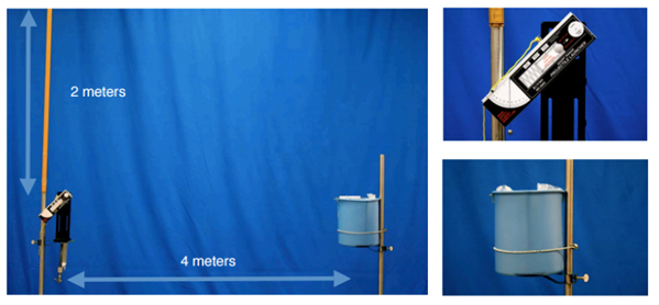
Figure 2. Experimental setup.

Representative results from steps 1 and 2 of the above procedure are listed below in Table 1. This table records the maximum height the ball reached in both 1 and 2 dimensions, with a known initial velocity and total flight time. The value of the experimentally measured maximum vertical displacement is compared to that calculated using Equation 15, the value of which is also found below. The table also records the maximum horizontal displacement of the ball for the 2-dimensional experiment. This is compared with the calculated value from Equation 13 using the known initial velocity and measured flight time. These two results match very well, which validates the kinematic equations.

Calculated Flight Time (s)	Calculated y (m)	Average Measured Flight time (s)	Average Measured y (m)
1.28	2.02	1.22	2.1

Table 1. Calculated and measured results in one dimension.

Calculated Flight Time (s)	Calculated y (m)	Calculated x (m)	Average Measured Flight time (s)	Average Measured y (m)	Average Measured x (m)
0.9	1.01	4.01	1.02	1.1	4

Table 2. Calculated and measured results in two dimensions.

Kinematics is used in a wide range of applications. The military uses these kinematic equations to determine the best way to launch ballistics. For better accuracy, the drag of air resistance is included in the equations. Car manufactures use kinematics to figure out top speeds and stopping distances. In order to take off,airplanes must attain a certain speed before they run out of runway. With kinematics,it is possible compute how fast the pilot will need to accelerate when taking off at a certain airport.