Material Constants

Source: Roberto Leon, Department of Civil and Environmental Engineering, Virginia Tech, Blacksburg, VA

In contrast to the production of cars or toasters, where millions of identical copies are made and extensive prototype testing is possible, each civil engineering structure is unique and very expensive to reproduce (Fig.1). Therefore, civil engineers must extensively rely on analytical modeling to design their structures. These models are simplified abstractions of reality and are used to check that the performance criteria, particularly those related to strength and stiffness, are not violated. In order to accomplish this task, engineers require two components: (a) a set of theories that account for how structures respond to loads, i.e., how forces and deformations are related, and (b) a series of constants that differentiate within those theories how materials (e.g. steel and concrete) differ in their response.

Figure 1: World Trade Center (NYC) transportation hub.

Most engineering design today uses linear elastic principles to calculate forces and deformations in structures. In the theory of elasticity, several material constants are needed to describe the relationship between stress and strain. Stress is defined as the force per unit area while strain is defined as the change in dimension when subjected to a force divided by the original magnitude of that dimension. The two most common of these constants are the modulus of elasticity (E), which relates the stress to the strain, and Poisson's ratio (ν), which is the ratio of lateral to longitudinal strain. This experiment will introduce the typical equipment used in a construction materials laboratory to measure force (or stress) and deformation (or strain), and use them to measure E and ν of a typical aluminum bar.

The most common model used for analysis is linear elasticity (Hooke's Law), which postulates that changes in force (F) are directly proportional to changes in dimension (Δ). In its most simple form in cases of uniaxial loading, force and deformation are related by a single constant (E), or the modulus of elasticity:

   (Eq. 1)

   (Eq. 2)

   (Eq. 3)

   (Eq. 4)

As described in the equations above, the stress and strain are engineering quantities, as opposed to true quantities. True quantities require one to measure the small but finite changes in local dimensions that occur as the forces are increased. Experimentally, this feat is very difficult to accomplish, even with recent advances in non-contact measuring technologies. For these calculations, one can assume those changes are negligible and use the original area (A₀) and length (L₀).

In order to determine the modulus of elasticity from the equations above, one must have a way of determining the changes in force and length as a specimen is loaded. In a crude experiment, one could use a bathroom scale and a ruler to accomplish these tasks. First, one could take a thick rubber band, measure its dimensions, and mark two points on the band separated by one inch. Next, one could place an open container on a scale and add water until the reading is ten pounds. One could then suspend the container with the rubber band and measure how much the two marks have separated. This measurement will give us all the data needed to calculate E for rubber since we have all the values needed to solve for E in Eqs. (2) through (4). However, there will be very large uncertainties and error associated with the measurement because of the very crude measurement device. Since the magnitude of strain needed to be measured for typical construction materials are on the order of 1x10^-6, far more accurate measurement devices are necessary to determine material constants experimentally. For most common engineering applications, these measurements are based on electrical resistance strain gages. As these devices will be used throughout the subsequent videos, a description of their operating principles will be given next.

A strain gage is a long looped wire embedded on a carrier matrix (Fig. 2). The strain gage is glued to the material being tested with a high strength epoxy. When the material is deformed, the wires will change in length and their resistance will change slightly as a result. When the gage is inserted as part of a Wheatstone bridge circuit, these changes can be detected as changes in voltage. The advent of digital measurement systems has considerably reduced background noise and other sources of error within the circuit, thereby improving the precision in which voltage changes can be measured today. The strain gage is calibrated using a constant known as a gage factor, so that its output is linearly related to strain for a given strain range under a given voltage input.

A strain gage measures the strain in only one direction. In order to obtain the complete state of stress at a point on a surface, a rosette strain gage, which is composed of three strain gages aligned at 45º to one another is needed (Fig. 3). With these measurements in three different directions, the entire state of stress on a surface can be defined by using principles like Mohr's circle to calculate maximum and minimum principal strains and stresses.

Figure 2: Strain gage.

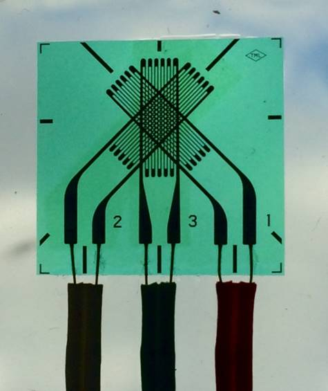
Figure 3: Rosette strain gage.

Measurements of force are also made with strain gages; however, these measurements are generally taken in a full bridge configuration (i.e., the internal resistances in a Wheatstone bridge circuit are replaced by external active gages) resulting in a device called a load cell. The load cell itself is usually a thick, high strength steel cylinder with two gages installed longitudinally and two installed transversely to eliminate the effects of Poisson's ratio. The calibration of a load cell requires that dead weights be used so that the voltage output of the circuit can be related to a given load. In the United States, the National Institute of Science and Technology (NIST) calibrates load cells up to 5 million kN using dead weights and lever mechanisms. All load cells used in the U.S. must be traceable to this calibration source. In practice, traceability means that load cell A is calibrated by NIST using dead weights, taken to other laboratories, and installed in series with load cell B. Finally, load cell B is calibrated based on comparing its output to the output of load cell A. All load cells must be periodically calibrated to ensure that they are working properly.

Typically, the load cell is installed on a universal testing machine (UTM). A UTM consists of a self-reacting frame with two screw columns that are turned by a motor (Fig. 4). By clamping a test specimen into the UTM grips and turning the screw column such that the crosshead moves upwards, tensile forces are introduced into the specimen. The applied force is measured by the load cell, which is installed in series with the specimen. On the other hand, if platens are installed instead of tensile grips and the screw columns are moved downward, compressive forces are introduced into the test specimen (i.e., to test concrete cylinders).

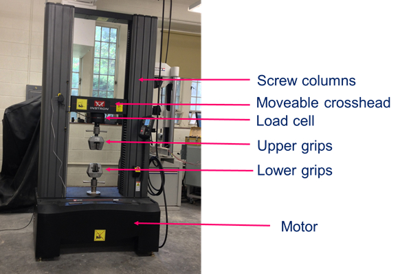
Figure 4: Universal testing machine.

Now that it has been demonstrated how to measure strain and force, a more general treatment of the theory of elasticity will be discussed. Looking at a generic piece of a structure subjected to loads, one can write equations of equilibrium for forces and moments along all axes.

This results in a series of equations for normal (ε) and shear (γ) strains of the form:

  (Eq. 5)

  (Eq. 6)

Six equations of this type, three for normal strains (ε_x, ε_y and ε_z) and three for shear strains (γ_xy, γ_yz and γ_zx) are needed to establish the global deformations. These equations contain three material constants: the modulus of elasticity (E), Poisson's ratio (ν), and the shear modulus (G). As shown in the equation above, the shear modulus is the change in angular deformation given a shear stress or surface traction. Poisson's ratio is defined as:

  (Eq. 7)

It can be shown that:

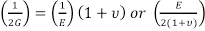= G  (Eq. 8)

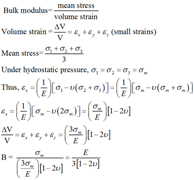
Thus, only two of the three constants need to be determined in order to define all three. There are numerous other derived constants that are used in elasticity theory, all of which can be derived from these measurements. For example, the bulk modulus (B), or the relative change in the volume of a body produced by a unit compressive or tensile stress acting uniformly over its surface, is:

From Eqs. (5) and (6), one can determine the state of stress and strain on a surface if at least three independent strain measurements are made. If a rosette strain gage, which has three gages at 45° to one another (Fig. 3) is used instead of a single longitudinal gage, then one can find the maximum and minimum principal strains (ε₁, ε₂) and the angle (Φ) between the measured strains and the principal strains from Mohr's circle.

For a rectangular rosette strain gage, such as that shown in Fig. 3 where the gages are at 45 degrees to one another:

(Eq. 9)

Φ =

The range of strains over which the linear elastic relationships hold is between zero and the proportional limit of the material. In this experiment, which will use aluminum, the range of strains will be kept well below that limit.

We will use a simple cantilever beam instrumented with strain gages to help illustrate the concepts of principal strain and stresses and the calculation of Young’s modulus (E) and Poisson’s ratio (ν).  The cantilever beam will be loaded incrementally with a set of weights and the corresponding changes in strain recorded.  The corresponding stresses can be calculated from the simple bending stress equation:

   (Eq. 11)

where M is the moment (or force multiplied by its lever arm), c is the distance from the centroid to the extreme fiber in the beam across its depth (), and I is the moment of inertia, given by   where b is the beam width and t is its thickness.

Modulus of Elasticity and Poisson's Ratio

It will be assumed herein that students have been trained in the use and safety precautions required to operate a universal testing machine.

1. Obtain a rectangular aluminum bar (12 in. x 1 in. x ¼ in.); an aluminum 6061 T6xxx or stronger is recommended. A hole should be drilled about 1 in. from one beam end to serve as a loading point.
2. Mark a location on the beam about 8.0 in. from the center of the hole on the top surface of the beam. Draw alignment marks for the rosette strain gages and make sure that the axes of the rosette are inclined at a small angle (about 10° to 15°) to the longitudinal axis of the beam.
3. Mark a similar location on the bottom surface of the beam. A single strain gage will be installed here and should be aligned with the longitudinal axes of the beam.
4. Measure width (b) and thickness (t) of the bar carefully using calipers. Perform three replicates at three different locations to obtain a good average of the dimensions. From these measurements, calculate the moment of inertia (I) and the distance from the neutral axis to the extreme fiber of the bar (c=t/2).
5. Obtain a rosette strain gage with a sensing grid of approximately ¼ in. long by 1/8 mm wide on each gage and a similar single strain gage. Note the calibration factors (or gage factor) for all the gages.
6. To install the rosette strain gage, first degrease and clean the surface carefully; sand the surface using progressively finer sandpaper until a very smooth surface is obtained; clean the surface with a neutralizer; and glue the strain gage according to the manufacturer's specifications. Allow the glue to cure properly before proceeding.
7. Test the resistance of the gages (typically 120 ohms) and their current leakage to the bar (resistivity, ideally greater than 5 Mohms) before proceeding.
8. Repeat steps 1.5 to 1.7 for the single gage to be installed on the lower surface.
9. Insert the specimen in the cantilever apparatus and secure appropriately.
10. Connect the strain gages to a recording device, such as a Vishay P3 strain indicator. Make sure that the wiring is correct as per the strain indicator instructions and that you know which channel corresponds to each strain gage.
11. Enter the appropriate gage factors for each gage in the indicator.
12. Check the device calibration by inputting a known voltage that will result in a reading of 5000με at a gage factor of 2.00.
13. Record initial load and strains.
14. Slowly apply 9 increments of 1.1 lbs (0.5kg) or similar at the beam end. Pause at every step and allow measurements to stabilize before recording readings.
15. Slowly apply 9 decrements of 1.1 lbs (0.5kg) or similar. Pause at every step and allow measurements to stabilize before recording readings.
16. Disconnect strain gage from strain indicator and turn the indicator off.
17. Plot the strain in the longitudinal gage vs. the strain in the transverse gage. The slope of this line corresponds to Poisson's ratio, v.
18. Determine the slope of the best fit line from the plot of stress vs. longitudinal strain, which is equal to Young's modulus, E.
19. Compare your values of E and v with previously established or published values (in general, there will be a range of values given rather than a single discrete value).

The data should be imported or transcribed into a spreadsheet for easy manipulation and graphing. The data collected is shown in Table 1.

Because the rosette strain gage is not aligned with the principal axes of the beam, the rosette strains need to be input into the equations for ε_1,2 (Eq. 9) and ε (Eq. 10) above to compute principal strains, resulting in the data shown in Table 2. The table shows that the angle between the measured stress and the principal stresses is about 0.239 radians or 13.7°. Note that the maximum principal strain is positive, corresponding to a large tensile strain longitudinally; the minimum principal strain is negative, corresponding to a smaller transverse compressive strain. The ratio between the minimum and maximum principal strains corresponds to Poisson's ratio, which is shown on the last column and averages about 0.310.

	Load	Gage 1	Gage 2	Gage 3	Gage 44
Step	(Lbs.)	με	με	με	με
1	0.00	1	1	1	0
2	1.10	83	56	-21	-87
3	2.21	163	115	-41	-171
4	3.31	243	171	-62	-254
5	4.42	325	228	-83	-338
6	5.52	400	280	-104	-423
7	6.62	485	338	-122	-501
8	7.73	557	386	-143	-589
9	8.83	634	442	-163	-665
10	9.93	714	502	-184	-741
11	8.83	637	445	-162	-664
12	7.73	561	391	-142	-584
13	6.62	483	335	-123	-506
14	5.52	406	281	-102	-423
15	4.42	323	227	-83	-339
16	3.31	245	171	-62	-256
17	2.21	164	115	-41	-170
18	1.10	83	56	-21	-87
19	0.00	1	0	1	2

Table 1: Strains in aluminum bar.

Gage Factor	1	2	3	Maximum Principal Strain	Minimum. Principal Strain	Angle	Poisson's Ratio
Load step	με	με	με	(Eq. 9)	(Eq. 9)	(Eq. 10)	(Eq. 7)
1	1	1	1	1	1	0	0
2	83	56	-21	89	-26	-0.223	0.297
3	163	115	-41	176	-55	-0.243	0.311
4	243	171	-62	263	-82	-0.242	0.312
5	325	228	-83	351	-109	-0.240	0.311
6	400	280	-104	432	-136	-0.240	0.314
7	485	338	-122	523	-160	-0.237	0.307
8	557	386	-143	600	-186	-0.236	0.310
9	634	442	-163	684	-213	-0.238	0.312
10	714	502	-184	773	-242	-0.242	0.314
11	637	445	-162	688	-213	-0.239	0.309
12	561	391	-142	605	-186	-0.237	0.308
13	483	335	-123	520	-161	-0.236	0.309
14	406	281	-102	437	-133	-0.234	0.303
15	323	227	-83	349	-109	-0.241	0.313
16	245	171	-62	264	-81	-0.238	0.308
17	164	115	-41	177	-54	-0.239	0.302
18	83	56	-21	89	-26	-0.223	0.297
19	1	0	1	2	0	0.000	0.000
					Average	-0.239	0.310

Table 2: Principal strains and angle of inclination.

The maximum and minimum principal strains from Table 2 are plotted in Fig. 5 which shows very linear trends (R² = 0.999) for Poisson's ratio. The value obtained for Poisson's ratio (0.31), which corresponds to the slope of the line, is very close to the 0.30 given in most references for aluminium and other metals.

Figure 5: Principal strain data showing the slope of the line between maximum and minimum principal strain, which corresponds to Poisson's ratio.

A good physical interpretation of the rosette strain gage data can be gained from plotting the principal strains on a Mohr circle (Fig. 6). Note that the three measurements, shown here for the case of the maximum load of 7.4 lbs., correspond to three points in the circle at 90º to one another, starting at an angle of about 27.4º (or 2Φ) counterclockwise from the x-axis.

Figure 6: Physical significance of strain rosette readings shown on Mohr's circle for strain.

Table 3 shows the loads, the results for the principal tensile strain from the single gage on the underside of the beam (Gage 4, which is in compression), the ratio between the bottom and top maximum principal stresses, the stress from Eq. (11), and Young's modulus (E) as the ratio of the stress from Eq. (11) divided by the strain from Eq. (9). In Table 3, a Young's modulus is calculated as 10147 ksi by taking the average of the moduli calculated for the 15 intermediate loading steps.

	Load	Max. Principal. Strain	Max Principal Stress	Min Principal Stress	Bending Stress	Young' Modulus
Load step	Lbs.	με	ksi	ksi	psi	ksi
1	0.00	1	10	9	0	0
2	1.10	89	886	0	882	9945
3	2.21	176	1765	0	1763	9991
4	3.31	263	2630	0	2645	10058
5	4.42	351	3513	0	3526	10038
6	5.52	432	4324	0	4408	10195
7	6.62	523	5230	0	5290	10113
8	7.73	600	6001	0	6171	10283
9	8.83	684	6843	0	7053	10307
10	9.93	773	7726	0	7935	10269
11	8.83	688	6877	0	7053	10256
12	7.73	605	6051	0	6171	10198
13	6.62	520	5204	0	5290	10165
14	5.52	437	4368	0	4408	10091
15	4.42	349	3494	0	3526	10092
16	3.31	264	2644	0	2645	10004
17	2.21	177	1770	0	1763	9960
18	1.10	89	886	0	882	9945
19	0.00	2	19	0	0	0
					Average	10147

Table 3: Calculation of modulus of elasticity (E).

The data for E is also plotted in Fig. 7, which indicates an excellent linear relationship (high R²) between stress and strain and a slope of about 10,147 ksi. The difference between the modulus from Table 3 and that from Fig. 6 arises because the calculations for the slope in Fig. 6 require that the intercept go through zero. The magnitudes compare very favourably (error less than 1.5%) with published values of E for 6061T6 aluminium, which is usually given as 10,000 ksi.

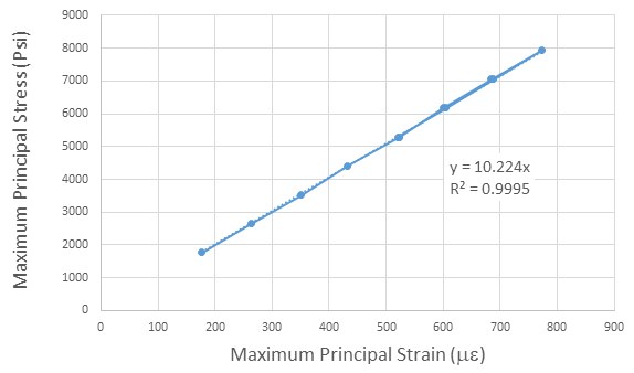
Figure 7: Slope of line of maximum stress vs. maximum strain is Young's modulus.

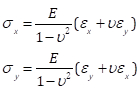
Finally, by recasting Eqs. (5) and (6) into:

(Eq. 12)

we can calculate the principal stresses using Mohr's circle. For the case of the step corresponding to 6.61 lbs. of load, the principal strains of (634, -189) lead to principal stresses of (7.34, 0.00) ksi (Fig. 8). Although the calculations here are done using the expressions for plane stress, the results correctly indicate that along the principal axis the stress in the perpendicular direction is zero (or very close to it), corresponding to the case of uniaxial loading. The stress values at an angle of 2Φ = 0.40 radians are (6.50, 2.82) ksi.

Figure 8: Mohr's circle for plane stress for the case of a 7.34 lbs load.

In this experiment, two fundamental material constants were measured: the modulus of elasticity (E) and Poisson's ratio (v). This experiment demonstrates how to measure these constants in a laboratory setting using a rosette strain gage. The values obtained experimentally match well with the published values of 10,000 ksi and 0.3, respectively. These values are key in applying the theory of elasticity for engineering design, and this experimental technique described herein are typical of those used for obtaining materials constants. To obtain these values, great care must be taken both in utilizing high resolution instrumentation and traceable calibration procedures. In particular, the use of strain gage-based devices and 16 to 24-bit digital data acquisition systems are integral to the success and quality of such experiments.

Today, there are other methods of determining Young's modulus of a material, including wave propagation methods (ultrasonic echo-pulse method) and nanoindentation. One benefit of utilizing wave propagation is that it is one of the non-destructive methods of measuring Young's modulus, whereas nanoindentation and use of a rosette strain gage are more invasive methods.

The design of any engineering product, from a toaster to a skyscraper, requires the use of effective analytical models to improve and optimize the design. The theory of elasticity is the foundation of most models used in civil engineering design, and is based upon the establishment of several constants.

Analytical models are required when only a single (or very few) replicates will be built. As the cost and performance of the structure depend on the result of those analyses, and those analyses, in turn, depend on having robust values for the material properties, tests such as the ones described here must be run to ensure quality control and quality assurance in the construction process. For example:

• In choosing a façade for a building, the architect must be careful to design a waterproof envelope. The water tightness of a brick building façade may depend on maintaining the mortar between the bricks uncracked, among other factors. If the mortar cracks, water will penetrate and cause corrosion and humidity problems which will be very expensive to fix. In order to determine how much force the mortar can resist before it cracks, we need both a theory and its associated constants. The architect and structural engineer must work together to determine what loads the façade will see (self-weight, wind, driving rain, etc.) and how each design option will perform under those conditions. Only then can a mortar with the appropriate characteristics should be chosen.
• In constructing a tall building, such as the Burj Dubai, the construction company needs to pay close attention to keeping the floors level. As the construction progresses, if the sizes of the columns and walls are different, some of these elements may shorten (strain) more than others as the construction progresses and more weight (stress) is added. To obtain flat floors at the end of construction, the construction company will need to make adjustments to the height of the columns and walls in the lower floors - the lower floors may not be level during the initial phases of construction but should be flat at the end. To calculate how to properly make these adjustments, the construction company will hire a structural engineer to provide data on differential column and wall heights. The engineer will need to use material constants to carry out these computations.
• In the design of a soda can, a manufacturer must minimize the thickness of the aluminum wall, as aluminum is a very expensive material. To optimize the shape and dimensions of the cans, the manufacturer needs to determine what loading conditions are important; transportation and storage conditions may be more demanding than the consumer drinking from it. Many of these conditions will be hard and expensive to replicate within an experimental testing program; the manufacturer may choose to do a lot of analysis to optimize the can dimensions before moving to the prototype phase. This procedure is what Boeing followed in developing the Dreamliner (Boeing 787). To do these studies, material properties must be known and the appropriate theory selected.