Cross Cylindrical Flow: Measuring Pressure Distribution and Estimating Drag Coefficients
Overview
Source: David Guo, College of Engineering, Technology, and Aeronautics (CETA), Southern New Hampshire University (SNHU), Manchester, New Hampshire
The pressure distributions and drag estimations for cross cylindrical flow have been investigated for centuries. By ideal inviscid potential flow theory, the pressure distribution around a cylinder is vertically symmetric. The pressure distribution upstream and downstream of the cylinder is also symmetric, which results in a zero-net drag force. However, experimental results yield very different flow patterns, pressure distributions and drag coefficients. This is because the ideal inviscid potential theory assumes irrotational flow, meaning viscosity is not considered or taken into account when determining the flow pattern. This differs significantly from reality.
In this demonstration, a wind tunnel is utilized to generate a specified airspeed, and a cylinder with 24 ports of pressure is used to collect pressure distribution data. This demonstration illustrates how the pressure of a real fluid flowing around a circular cylinder differs from predicted results based on the potential flow of an idealized fluid. The drag coefficient will also be estimated and compared to the predicted value.
Principles
The non-dimensional pressure coefficient, Cp, for an arbitrary position in ideal potential flow theory at any angular position, θ, on the surface of a circular cylinder is given by the following the equation:

The pressure coefficient Cp is defined as:
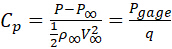
where P is the absolute pressure, P∞ is the undisturbed free-stream pressure, Pgage = P − P∞ is the gage pressure, and  is the dynamic pressure, which is based on the free-stream density, ρ∞, and airspeed, V∞.
The flow pattern predicted by ideal potential flow theory is shown in Figure 1. The flow is symmetrical, and therefore there is zero net drag force. This is called D'Alembert's Paradox [1].
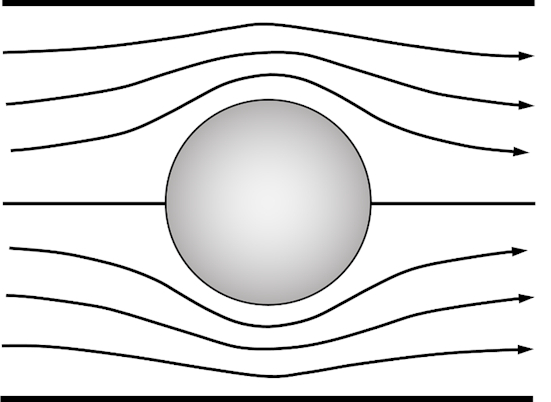
Figure 1. Flow pattern of an ideal cross-cylindrical flow in a wind tunnel.
However, a net zero drag force is not expected under real flow conditions. The drag force of a cylinder, FD, per unit length of the cylinder due to pressure differences is given by:

The integration is taken along the perimeter of the cylinder.
In this experiment, gage pressure measurements are collected from 24 pressure ports along the cylinder. Then, the above equation can be numerically evaluated using the measured gage pressure as follows:

where Pgagei is the gage pressure at the location of θi, θi is the angular position, r is the radius of the cylinder, and  θ is the angular distance between adjacent ports, which is 15°. The gage pressure is determined using a manometer panel with 24 independent columns, the gage pressure is determined using the following equation:

where Δh is the height difference of the manometer in reference to the free-stream pressure, ρL is the density of the liquid in the manometer, and g is the acceleration due to gravity. Once the drag force is obtained, the non-dimensional drag coefficient CD can be determined through:

where d = 2r is the diameter of the cylinder.
Remembering D'Alembert's Paradox, the drag force is due to the neglected effects of viscosity. First, a boundary layer develops along the cylinder as a result of viscous forces. These viscous forces cause skin-friction drag. Second, the cylinder is a bluff (non-streamlined) object. This creates flow separation and a low-pressure wake behind it and causes a larger drag force due to the pressure differential. Figure 2 displays several typical flow patterns that are observed experimentally. Real flow patterns rely on the Reynolds number, Re, which is defined as:
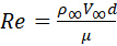
where the parameter μ is the dynamic viscosity of the fluid.

Figure 2. Various types of flow patterns over a cylinder.
Procedure
1. Measuring the pressure distribution around a cylinder
- Remove the top cover of the test section of a wind tunnel, and mount a clean, aluminum cylinder (d = 4 in) with 24 built-in ports on a turntable (Figure 3). Install the cylinder so that port zero is facing upstream (Figure 4a).
- Replace the top cover, and connect the 24 pressure tubes labeled 0 - 23 to the corresponding ports on the manometer panel. The manometer panel should be filled with colored oil but marked in water in. graduations (Figure 5).
- Turn on the wind tunnel and run it at 60 mph. Record all 24 pressure measurements by reading the manometer. At this airspeed, the Reynolds number is 1.78 x 10⁵. The expected flow pattern is shown in Figure 2d.
- Once all measurements have been recorded, turn off the wind tunnel and tape two strings (d = 1 mm) vertically on the cylinder to create the disturbed cylinder. Tape one string between ports 3 and 4 (θ = 52.5°) and the other between ports 20 and 21 (θ = 307.5°). Make sure the ports nearby are not blocked by the tape, as shown in Figure 4b.
- Turn on the wind tunnel, and repeat step 3. Record all pressure measurements.

Figure 3. Gage pressure measurement layout of cross cylindrical flow.
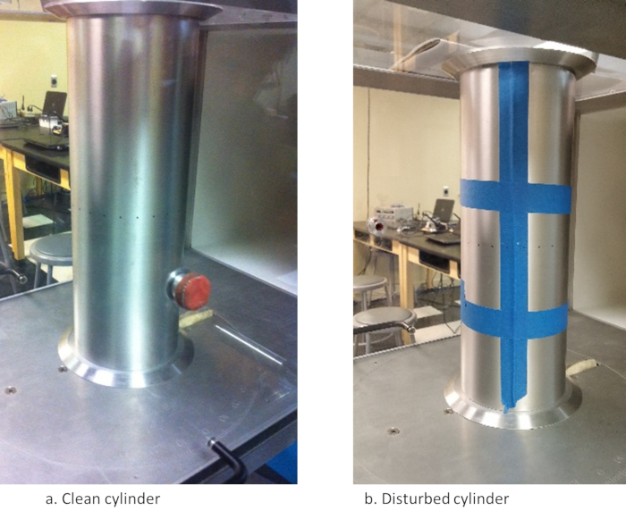
Figure 4. Setup of the cylinder in the wind tunnel (pressure ports are in the middle of the cylinder).
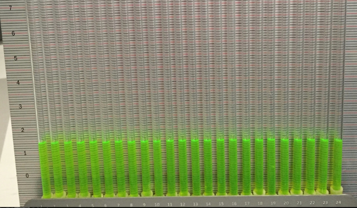
Figure 5. Manometer panel.
Results
Experimental results for the clean and disturbed cylinder are shown in Tables 1 and 2, respectively. The data can be plotted in a graph of the pressure coefficient, Cp, versus angular position, θ, for ideal and real flow as shown in Figure 6.
| Pressure port # | Position angle q (°) | Pgage from manometer readings (in. water) | Calculated pressure coefficient Cp |
| 0 | 0 | 1.7 | 1.00 |
| 1 | 15 | 1.4 | 0.83 |
| 2 | 30 | 0.0 | 0.01 |
| 3 | 45 | -1.7 | -0.98 |
| 4 | 60 | -2.7 | -1.57 |
| 5 | 75 | -3.7 | -2.15 |
| 6 | 90 | -3.3 | -1.92 |
| 7 | 105 | -3.0 | -1.74 |
| 8 | 120 | -3.2 | -1.86 |
| 9 | 135 | -3.2 | -1.86 |
| 10 | 150 | -3.3 | -1.92 |
| 11 | 165 | -3.5 | -2.03 |
| 12 | 180 | -3.4 | -1.97 |
Table 1. Experimental results for the clean cylinder. Due to symmetry, only data for ports number 0-12 are shown.
| Pressure port # | Position angle q (°) | Pgage from manometer readings (in. water) | Calculated pressure coefficient Cp |
| 0 | 0 | 1.8 | 1.05 |
| 1 | 15 | 1.6 | 0.93 |
| 2 | 30 | 0.6 | 0.35 |
| 3 | 45 | -1.3 | -0.73 |
| 4 | 60 | -2.9 | -1.69 |
| 5 | 75 | -4.0 | -2.31 |
| 6 | 90 | -4.0 | -2.33 |
| 7 | 105 | -1.7 | -0.99 |
| 8 | 120 | -1.5 | -0.89 |
| 9 | 135 | -1.4 | -0.84 |
| 10 | 150 | -1.4 | -0.84 |
| 11 | 165 | -1.5 | -0.87 |
| 12 | 180 | -1.4 | -0.84 |
Table 2. Experimental results for the disturbed cylinder. Due to symmetry, only data for ports number 0-12 are shown.

Figure 6. Pressure coefficient distribution, Cp, vs angular position, θ, between ideal and real flow.
At the stagnation point, θ = 0°, Cp reaches its maximum value of Cp = 1. For θ < 60°, the pressure coefficient distribution is similar for all three curves. This is where the laminar boundary layer flow is attached to the surface of cylinder. For θ > 60°, the two experimental flow patterns deviate from the ideal flow; they form a low-pressure region in the back of the cylinder, which is filled with turbulent vortices and eddies. This is the called the wake region. It is the pressure difference between the front and the back of the cylinder that causes the large drag that is observed in cross cylindrical flow.
Despite the similarity in flow patterns between the clean cylinder and disturbed cylinder, there are also differences. The disturbed flow tends to wrap around the cylinder more prior to flow separation, and it also has a higher back pressure. This causes less drag, which is verified by the drag calculations. This occurs because the laminar flow in the front of the cylinder has a tendency to flow straight and it is difficult for the flow to wrap around the cylinder. For the disturbed cylinder, the flow immediately transitions into turbulent flow and thus can wrap around the cylinder more than the clean cylinder.
| Flow Configurations | Drag coefficient, CD |
| 1. Clean cylinder | 1.68 |
| 2. Disturbed cylinder | 0.78 |
Table 4. Drag coefficient, CD (Reynolds number Re = 1.78 x 10⁵).
The drag coefficient CD for clean cylinder at 60-mph airspeed or Re = 178,000 has been evaluated experimentally and is approximately 1.5 [2], which is close to the value of 1.68 that was obtained in this experiment for a clean cylinder.
From previous experimental results [2], the drag coefficient CD drops at Re = 3 x 10⁵. This is because the transition from laminar flow to turbulent flow occurs naturally even with a smooth cylinder. In the experiment, the turbulent flow transition is observed by simply taping a 1-mm diameter string to the surface of the cylinder. Thus, a lower drag coefficient CD of only 0.78 is obtained for the disturbed cylinder.
Application and Summary
Cross cylindrical flow has been investigated theoretically and experimentally since the 18th century. Finding the discrepancies between the two allows us to expand our understanding of fluid dynamics and explore new methodologies. Boundary layer flow theory was developed by Prandtl [3] in early 20th century, and it is a good example of the extension of inviscid flow to viscid flow theory in solving D’Alembert’s Paradox.
In this experiment, the cross cylindrical flow was investigated in a wind tunnel and the 24 ports of pressure measurement were made to find the pressure distribution along the surface of the cylinder. The drag coefficient was calculated and it agrees well with other sources. The manipulation of the flow to trigger turbulent boundary flow at relative low Reynolds number was also demonstrated.
References
- d'Alembert, Jean le Rond (1752), Essai d'une nouvelle théorie de la résistance des fluides
- John D. Anderson (2017), Fundamentals of Aerodynamics, 6th Edition, ISBN: 978-1-259-12991-9, McGraw-Hill
- Prandtl, Ludwig (1904), Motion of fluids with very little viscosity, 452, NACA Technical Memorandum
Tags
Skip to...
Videos from this collection:

Now Playing
Cross Cylindrical Flow: Measuring Pressure Distribution and Estimating Drag Coefficients
Aeronautical Engineering
16.2K Views

Aerodynamic Performance of a Model Aircraft: The DC-6B
Aeronautical Engineering
8.3K Views

Propeller Characterization: Variations in Pitch, Diameter, and Blade Number on Performance
Aeronautical Engineering
26.3K Views

Airfoil Behavior: Pressure Distribution over a Clark Y-14 Wing
Aeronautical Engineering
21.0K Views

Clark Y-14 Wing Performance: Deployment of High-lift Devices (Flaps and Slats)
Aeronautical Engineering
13.3K Views

Turbulence Sphere Method: Evaluating Wind Tunnel Flow Quality
Aeronautical Engineering
8.7K Views

Nozzle Analysis: Variations in Mach Number and Pressure Along a Converging and a Converging-diverging Nozzle
Aeronautical Engineering
37.9K Views

Schlieren Imaging: A Technique to Visualize Supersonic Flow Features
Aeronautical Engineering
11.4K Views

Flow Visualization in a Water Tunnel: Observing the Leading-edge Vortex Over a Delta Wing
Aeronautical Engineering
8.0K Views

Surface Dye Flow Visualization: A Qualitative Method to Observe Streakline Patterns in Supersonic Flow
Aeronautical Engineering
4.9K Views

Pitot-static Tube: A Device to Measure Air Flow Speed
Aeronautical Engineering
48.8K Views

Constant Temperature Anemometry: A Tool to Study Turbulent Boundary Layer Flow
Aeronautical Engineering
7.2K Views

Pressure Transducer: Calibration Using a Pitot-static Tube
Aeronautical Engineering
8.5K Views

Real-time Flight Control: Embedded Sensor Calibration and Data Acquisition
Aeronautical Engineering
10.2K Views

Multicopter Aerodynamics: Characterizing Thrust on a Hexacopter
Aeronautical Engineering
9.1K Views
Copyright © 2025 MyJoVE Corporation. All rights reserved