Optical Materialography Part 2: Image Analysis

Morphological information from the internal three-dimensional structure of a material can be obtained by applying materialographical techniques, that is, techniques that do a statistical analysis of carefully chosen two-dimensional sections, to optical microscope images.

The porosity in a material, which is the fraction of the volume of a material that is open space (not occupied by atoms), can determine its mechanical, electrical, optical properties and directly affects mass transport through it (its permeability). Porosity as a volume fraction can be shown to be statistically equivalent to the area fraction or point fraction of voids in a representative two-dimensional slice:

  [1]

  [2]

where A_A is the area of void area, normalized by the total imaged area, and P_P is, likewise, the number of points lying in void divided by the total probe points. The brackets indicate an average over multiple samples.

The average grain size, the average lateral dimension of a crystal grain in a polycrystalline material, can be quantified by measuring the mean intercept grain size, G, which can be determined by overlaying test lines on the microstructural image:

  [3]

where I_L is the number of intersections between the test lines (see Figure 2) and the grain boundaries per unit test line length. For high porosity materials, G can be found by:

  [4]

Finally, the effective density of a material can be calculated by taking the porosity, measured by the materialographic techniques, into consideration. This Effective Density, takes into account the volume of the pores in a material, whereas the 'density' may refer only to the non-porous region (depending on the measurement method). This effective density of the material can be found using:

  [5]

where Porosity can be obtained by <P_p> or, <A_A>.

In Figure 1 we see a cross section of a porous material with a grid superimposed on it. The points of intersection can be used to determine <P_p>. The number of intersection points that lie over dark regions (pores) is divided by the total number of intersection points to get P_p and by collecting and, by averaging P_p values from multiple images, we arrive at <P_p>.

Figure 1: Materialographic image with a superimposed grid. The intersection points on the grid are used for analysis.

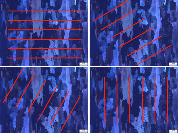
Figure 2: Grains size measurements using lines at a) 0, b) 30, c) 60 and d) 90 degrees orientation. The grains are obviously anisotropic in shape (longer in one direction than the other). This anisotropy results from the nonuniform forces acting on the samples during processing through which the grains become "squashed".

Image ID	Test points in porosity area	Total no. of test points	PP	<PP>
				Avg.	Δ*
P1	32	100	0.32	29	1.77
P2	29	100	0.29
P3	22	100	0.22
P4	37	100	0.37
P5	24	100	0.24
P6	30	100	0.30

Table 1. Porosity measurements.

ID	Probe L(mm)		Horizontal (Radial or Hoop)					Vertical (Axial)
			I	IL	<IL>		G	I	IL	<IL>		G
					Avg.	Δ
										Avg.	Δ*
SL1	0.9		16	17.7	18.1	0.68	0.05mm	3	3.33	3.7	0.31	0.27 mm
SL2	0.9		14	15.5				2	2.22
SL3	0.9		18	20				4	4.44
SL4	0.9		16	17.7				3	3.33
SL5	0.9		15	16.7				5	5.56
SL6	0.9	19		21.1				3	3.33

Table 2. Intercept measurements using straight line probes.

*: Δ is the sampling error. Assuming a confidence level of 95%, the sampling error can be estimated with the equation below:

N: number of samples

x_i: the i th sample

µ: sample average

The probability of population average lying in the range [µ- Δ, µ+ Δ] is 95%. The sampling error can be used as criteria in telling if the difference between two averages is significant (e.g. the difference between the average of I_L estimated with vertical line probes and horizontal line probes).

These are standard methods for analyzing two-dimensional cross sections in materials in order to extract three-dimensional information. We looked specifically at estimating the volume fraction of pores in one material and the average grain size in a second material.

Materialographic sample preparation described here are the necessary first step towards the analysis of internal microstructure of three-dimensional materials using two dimensional information. For example, one might be interested in knowing how porous a membrane material is since that will affect its gas pearmeability. An analysis of the void structure of the 2D cross section will provide a strong indication of what the porosity is in the actual 3D structure (provided the sampling statistics are high). Another application would be in analyzing, for example the orientation of the polycrystalline grains in oil pipeline alloys. The orientational distribution function (ODF) can be directly related to the axial and transverse mechanical strength of the pipes, and so our sample preparation procedure is an important component of such an analysis.