
Piping Networks and Pressure Losses
Overview
Source: Alexander S Rattner, Department of Mechanical and Nuclear Engineering, The Pennsylvania State University, University Park, PA
This experiment introduces the measurement and modeling of pressure losses in piping networks and internal flow systems. In such systems, frictional flow resistance from channel walls, fittings, and obstructions causes mechanical energy in the form of fluid pressure to be converted to heat. Engineering analyses are needed to size flow hardware to ensure acceptable frictional pressure losses and select pumps that meet pressure drop requirements.
In this experiment, a piping network is constructed with common flow features: straight lengths of tubing, helical tube coils, and elbow fittings (sharp 90° bends). Pressure loss measurements are collected across each set of components using manometers - simple devices that measure fluid pressure by the liquid level in an open vertical column. Resulting pressure loss curves are compared with predictions from internal flow models.
Principles
When fluid flows through closed channels (e.g., pipes, tubing, blood vessels) it must overcome frictional resistance from the channel walls. This causes a continual loss of pressure in the flow direction as mechanical energy is converted to heat. This experiment focuses of measurement and modeling of such pressure losses in internal flow systems.
To measure pressure drop along channels, this experiment will use the principle of hydrostatic pressure variation. In stationary fluid, pressure only varies with depth due to fluid weight (Eqn. 1, Fig. 1a).
 (1)
(1)
Here  and
and  are the pressures at two points, ρ is the fluid density, g is the gravitational acceleration, and h1 and h2 are the depths (measured in the direction of gravity) of the points from a reference level. At typical ambient conditions, the density of water is ρw = 998 kg m-3 and the density of air is ρa = 1.15 kg m-3. Because ρa << ρw, hydrostatic pressure variations in air can be neglected compared with liquid hydrostatic pressure variations, and the ambient atmospheric pressure can be assumed uniform (Patm ~ 101 kPa). Following this principle, the pressure drop along a channel flow can be measured by the difference in fluid levels in vertical open-top tubes connected to the channel:
  (Fig. 1b). Such liquid-level-based pressure measurement devices are called manometers.
The pressure loss along a length of a channel can be predicted with the Darcy friction factor formula (Eqn. 2). Here,  is the pressure loss along a length (L) of channel with internal diameter D. U is the average channel velocity, defined as the volume flow rate of fluid (e.g., in m3 s-1) divided by the channel cross-section area (e.g., in m2,
  for circular channels). f is the Darcy friction factor, which follows different trends for different channel geometries and flow rates. In this experiment, friction factors will be measured experimentally for straight and helically coiled lengths of tube, and compared with previously published formulas.
 (2)
(2)
Channel-flow friction factor trends depend on the Reynolds number (Re), which measures the relative strength of effects from fluid inertia to effects from fluid viscosity (frictional effects). Re is defined as  , where
  is fluid dynamic viscosity (~0.001 kg m-1 s-1 for water at ambient conditions). At low Re (
 2000 in straight channels), viscous effects are strong enough to damp out eddies in the flow, leading to smooth laminar flow. At higher Re (
 2000), random eddies can form in the flow, leading to turbulent behavior. Commonly used friction factor models for straight circular channel flows are presented in Eqn. 3.
 (3)
(3)
When fluid flows through helical tube coils, secondary internal vortices form (Fig. 1c). As a result, the friction factor  also depends on the Dean number, which accounts for the relative influence of tube curvature:
  . Here R is the radius of the tube coil, measured from the central axis to halfway into the tubing. A common correlation for is:
 (4)
(4)
Pipe fittings, valves, expansions/contractions, and other obstructions also cause pressure losses. One approach to model such minor losses is in terms of the equivalent length of plain channel required to yield the same pressure drop (Le/D). Here, and  are the friction factor and flow velocity in the inlet / outlet channel lengths (Fig 1d).
 (5)
(5)
Tables of representative equivalent channel lengths are reported in handbooks for common plumbing components (c.f., [1]). This experiment will measure the equivalent lengths for sharp 90°-bend fittings (elbows). Typical reported equivalent lengths for such fittings are Le/D ~ 30.
Procedure
1. Fabrication of piping system (see schematic and photograph, Fig. 2)
- Affix (tape or glue) a small plastic water reservoir to the work surface. If it is a covered container, drill holes in the lid for the inlet and outlet water lines and pump power cable.
- Mount the small submersible pump in the reservoir.
- Mount the rotameter (water flow meter) vertically in the work area. It may help to strap the rotameter to a small vertical beam or L-bracket to keep it upright. Connect a flow tube from the pump outlet to the rotameter inlet (lower port).
- Connect plastic compression fitting tees to both ends of a section of rigid plastic tube (recommend length L ~ 0.3 m, inner tube diameter D ~ 6.4 mm). Mount the tees on pipe clamps. Connect rubber tubing from one tee (inlet) to the rotameter outlet. Connect rubber tubing from the other tee (outlet) to the reservoir.
- Construct a second assembly with two mounted tee fittings. Wrap a length of soft plastic tubing coiled helically around a cylindrical core (recommend cardboard tube, R ~ 30 mm and ~5 tubing wraps). Zip ties or clamps may help keep the tubing coiled. Install the two free ends of the tubing to the tee fittings.
- Construct a third assembly with two mounted tee fittings. Connect four (or more) elbows with short lengths of rigid plastic tube between the tees. Using multiple elbows amplifies the pressure drop reading, improving measurement accuracy.
- Install clear rigid plastic tubes (~0.6 m) to the open ports on the six tee fittings. Use a level to ensure that the tubes are vertical. These tubes will be the manometers (pressure measurement devices).
- Fill the reservoir with water.
2. Operation
- Straight tube: Turn on the pump, and adjust the rotameter valve to vary the water flow rates. For each case, record the water flow rate and the vertical water level in each manometer tube. Record the pressure drop based on the difference in manometer levels (Eqn. 1).
- Coiled tube: Connect the coiled test section inlet to the rotameter outlet, and the test section outlet to the reservoir. As in Step 2.1, record the water flow rate and pressure drops for a number of flow rates.
- Elbow fittings: Connect the elbow fitting test section to the rotameter and reservoir. Collect a set of flow rate and pressure measurements, as in Step 2.2.
3. Analysis
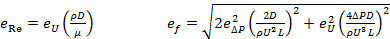
- For the straight tube case, evaluate the Reynolds number and friction factor f (Eqn. 2). Evaluate the Reynolds number and friction factor uncertainties (Eqn. 6). Here eΔP is the uncertainty in pressure measurements (
 ,
,  is uncertainty in manometer level), and eU is the uncertainty in average channel velocity (from rotameter data sheet, with typical uncertainty of 3 - 5% of range). For water at room temperature (22°C), ρ = 998 kg m-3 and µ = 0.001 kg m-1 s-1.
 (6)
(6) - Compare the friction factor results from Step 3.1 with the analytic models (Eqn. 3).
- Repeat Step 3.1 for the coiled tube case. This time, subtract the predicted pressure drop (Eqns. 2-3) for the straight portion of the test section from ΔP. Here we assume the uncertainty in the straight-length pressure correction is negligible. Compare measured friction factors with values from the correlation (Eqn. 4).
- Repeat Step 3.2 for the elbow fitting case. Subtract the predicted pressure drop for the straight lengths of tubing between the elbow fittings to obtain a corrected pressure loss
 . Evaluate the equivalent length and uncertainty for each elbow. Here, Ne is the number of pipe elbows.
 (7)
(7) - Compare the equivalent length result (Le/D) with the typical reported values (~30).
Results
Measured friction factor and equivalent length data are presented in Fig. 3a-c. For the straight tube section, a clear PVC tube with D = 6.4 mm and L = 284 mm is used. Measured flow rates (0.75 - 2.10 l min-1) correspond to turbulent conditions (Re = 2600 - 7300). Friction factors match predictions from the analytic model to within experimental uncertainty. Relatively high f uncertainty is found at low flow rates due to the limited accuracy of the selected (low-cost) flow meter (± 0.15 l min-1).
Friction factor results for the tube coil case also match the provided correlation (Eqn. 4) within experimental uncertainty (Fig. 3b). Five coil loops of radius R = 33 mm with tube inner diameter D = 6.4 mm are employed. Here, the Dean number is 500 - 5600, which corresponds to the laminar portion of Eqn. 4. Measured friction factors are significantly higher than for the straight section at equal flow rates. This stems from the stabilizing effect of the coil tube geometry, which delays the transition to turbulence to high Re.
For the elbow case, 4 elbow fittings (part number in materials list) are employed, connected by short lengths of D = 6.4 mm tubing. The equivalent frictional length of each elbow fitting approaches (Le/D) ~ 30 - 40 at high Re (Fig. 3c). This is similar to a commonly reported value of 30. Note that the actual frictional resistance is specific to the fitting geometry, and reported Le/D values should only be considered as guidelines.
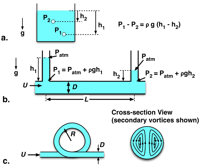
Figure 1: a. Schematic of hydrostatic pressure variation in a stationary body of fluid. b. Pressure change along a straight length of tube, measured with open-top manometers. c. Schematic of coiled tube, with internal vortices indicated in cross-section view.
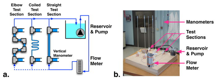
Figure 2: (a) Schematic and (b) photograph of pressure drop measurement facility. Please click here to view a larger version of this figure.

Figure 3: Friction factor and equivalent length measurements and model predictions for: a. Straight tube, b. Coiled tube, c. Elbow fittings.
Application and Summary
Summary
This experiment demonstrates methods for measuring pressure-drop friction factors and equivalent lengths in internal flow networks. Modeling methods are presented for common flow configurations, including straight tubes, coiled tubes, and pipe fittings. These experimental and analysis techniques are key engineering tools for the design of fluid flow systems.
Applications
Internal flow networks arise in numerous applications including power generation plants, chemical processing, flow distribution inside heat exchangers, and blood circulation in organisms. In all cases, it is critical to be able to predict and model pressure losses and pumping requirements. Such flow systems can be decomposed into sections of straight and curved channels, connected by fittings or junctions. By applying friction factor and minor loss models to such components, whole network descriptions can be formulated.
Materials List
| Name | Company | Catalog Number | Comments |
| Equipment | |||
| Submersible water pump | Uniclife | B018726M9K | |
| Covered plastic container | Water reservoir, plastic food container used in this study. | ||
| Water flow meter | UXCell | LZM-15 | Rotameter, 0.5 – 4.0 l min-1 |
| Rigid clear PVC tube | McMaster | 53945K13 | For test sections and manometers, 1/4” ID, 3/8” OD |
| Flexible soft PVC tubing | McMaster | 5233K63
5233K56 |
For tubing connections and coil test section |
| Plastic tube fitting tee | McMaster | 5016K744 | For test sections inlet and outlet connections/manometers |
| Plastic tube fitting elbow | McMaster | 5016K133 | For test section with elbows |
Skip to...
Videos from this collection:

Now Playing
Piping Networks and Pressure Losses
Mechanical Engineering
58.9K Views

Buoyancy and Drag on Immersed Bodies
Mechanical Engineering
30.2K Views

Stability of Floating Vessels
Mechanical Engineering
23.3K Views

Propulsion and Thrust
Mechanical Engineering
22.1K Views

Quenching and Boiling
Mechanical Engineering
8.2K Views

Hydraulic Jumps
Mechanical Engineering
41.3K Views

Heat Exchanger Analysis
Mechanical Engineering
28.3K Views

Introduction to Refrigeration
Mechanical Engineering
25.0K Views

Hot Wire Anemometry
Mechanical Engineering
15.9K Views

Measuring Turbulent Flows
Mechanical Engineering
13.6K Views

Visualization of Flow Past a Bluff Body
Mechanical Engineering
12.3K Views

Jet Impinging on an Inclined Plate
Mechanical Engineering
10.8K Views

Conservation of Energy Approach to System Analysis
Mechanical Engineering
7.4K Views

Mass Conservation and Flow Rate Measurements
Mechanical Engineering
23.0K Views

Determination of Impingement Forces on a Flat Plate with the Control Volume Method
Mechanical Engineering
26.0K Views
Copyright © 2025 MyJoVE Corporation. All rights reserved