
Measuring Turbulent Flows
Overview
Source: Ricardo Mejia-Alvarez and Hussam Hikmat Jabbar, Department of Mechanical Engineering, Michigan State University, East Lansing, MI
Turbulent flows exhibit very high frequency fluctuations that require instruments with high time-resolution for their appropriate characterization. Hot-wire anemometers have a short enough time-response to fulfill this requirement. The purpose of this experiment is to demonstrate the use of hot-wire anemometry to characterize a turbulent jet.
In this experiment, a previously calibrated hot-wire probe will be used to obtain velocity measurements at different positions within the jet. Finally, we will demonstrate a basic statistical analysis of the data to characterize the turbulent field.
Principles
A description of a turbulent flow
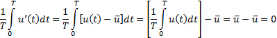
A turbulent flow can be evidenced by highly random fluctuations in flow variables such as velocity, pressure, and vorticity. Figure 1 represents a typical velocity signal obtained by measuring velocity at a fixed point in a turbulent flow. The fluctuations in this signal are not random noise, but the result of non-linear interactions between coherent motions within the flow field. A classical description of turbulent flow, involves the determination of the average value of flow variables and their corresponding fluctuations as time progresses. To this end, we use the definition for the average of a function to determine the average of a velocity measurement:
 (1)
(1)
Here,  is the size of the integration domain, which will be a time interval in the present measurements. As hinted by equation (1), we will use an overbar to denote the average of a variable. Given that a digital acquisition of a signal is discrete, the integral in equation (1) should be solved numerically, using either the trapezoidal or the Simpson's rule [1]. The fluctuations of a time-dependent variable like
  can then be calculated as follows:
 (2)
(2)
As seen in this equation, fluctuation fields are denoted by a prime symbol. By applying equation (1) to  , we can easily determine that the average of a fluctuation field is zero:
 (3)
(3)
Hence, a more appropriate statistical descriptor for the fluctuation field is the root mean square of the fluctuations:
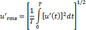 (4)
(4)
This statistical descriptor is in fact a very common measure of the turbulence intensity. The current experiment will be based on determining the average velocity and turbulence intensity of a turbulent field.
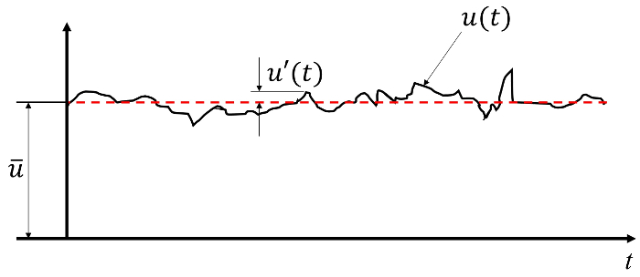
Figure 1. Typical signal of velocity of a turbulent flow as recovered by a hot-wire anemometer. The raw signal,  , can be decomposed in a fluctuation field,
  , superimposed on the average value of velocity,
  .
.
Experimental setup
As shown in Figure 2(A) the facility is basically a plenum that gets pressurized by a centrifugal fan. Figure 2(B) shows that there is a slit on the opposite side of the plenum that issues a planar jet. As shown in Figure 2(C), a traversing system holds the hot-wire anemometer at prescribed locations in the planar jet. This traversing system will be used to determine the velocity at different positions of interest in the jet. The schematic of Figure 3 shows a representative location at which anemometry will be carried out in order to characterize the turbulent field in the planar jet.
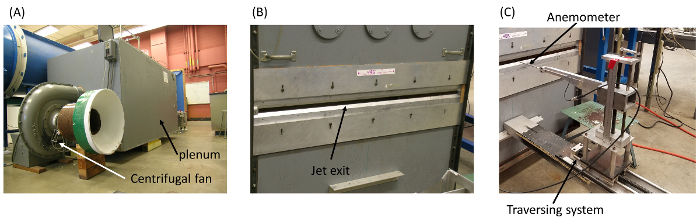
Figure 2. Experimental setup. (A): flow facility; the plenum is pressurized by means of a centrifugal fan. (B): slit for issuing the planar jet. (C): traversing system to change the position of the anemometer along the jet. Please click here to view a larger version of this figure.

Figure 3. Schematic of the planar jet showing: the vena contracta, the velocity distribution at a given downstream position, and the diagram of connections. Please click here to view a larger version of this figure.
Procedure
- Measure the width of the slit, W, and record this value in table 1.
- Set the hot-wire anemometer at a distance from the exit equal to x = 1.5W along the centerline. Record this streamwise position in table 2. The centerline is the origin of the spanwise coordinate (y = 0).
- Start the data acquisition program for traversing the jet. Set the sample rate at 500 Hz for a total of 5000 samples (i.e. 10s of data).
- Record the current spanwise position of the hot-wire in table 3.
- Acquire data.
- The data acquisition system will calculate the average velocity and turbulence intensity of that dataset using equations (1) and (4).
- Record those two values in table 3.
- Move the hotwire to the next (positive) spanwise position (
 mm).
mm). - Repeat steps 5 to 8 until there is not any noticeable change on both the average velocity and the turbulence intensity.
- Move the hot-wire back to the centerline.
- Move the hotwire to the next (negative) spanwise position (
 mm).
mm). - Acquire data.
- The data acquisition system will calculate the average velocity and turbulence intensity of that dataset using equations (1) and (4).
- Record those two values in table 3.
- Repeat steps 11 to 14 until there is not any noticeable change on both the average velocity and the turbulence intensity.
- Move the hot-wire back to the centerline of the jet.
- Move the hot-wire along the centerline of the jet in the downstream direction to a new position (e.g. x = 3W).
- Repeat steps 4 to 17 for as many streamwise positions as wanted (e.g. x = 1.5W, 3W, 6W, 9W).
Table 1 . Basic parameters for experimental study.
| Parameter | Value |
| Slit width (W) | 19.05 mm |
| Air density (r) | 1.2 kg/m3 |
| Transducer calibration constant (m_p) | 76.75 Pa/V |
| Calibration constant A | 5.40369 V2 |
| Calibration constant B | 2.30234 V2(m/s)-0.65 |

Figure 4. Flow control in the flow system. The stack on top of the plenum serves the purpose of diverting flow from the jet slit allowing to control the jet ' s exit velocity. Please click here to view a larger version of this figure.
Results
Figure 5 shows the distribution of average velocity across the jet at the downstream position x = 3W. And Figure 6 shows the distribution of turbulence intensity across the jet at the same downstream position. Table 3 has the results for the local values of average velocity and turbulence intensity at the streamwise position x = 3W. The last column of this table is the ratio between the local velocity and the centerline velocity. This ratio is used to determine the jet width,  , which is defined as the distance between the two positions at which the local velocity is 50% of the centerline velocity. Note from table 2 that these two positions are somewhere in the intervals
  and
and  . Their exact locations are determined using linear interpolation, and are determined to be:
  mm and
  mm, for a jet thickness of
  mm.
mm.
The results for four different experiments are compared in table 2. This table shows how the centerline velocity of the jet,  , remains basically unchanged for
  , but decreases with
  for
for  . This effect is the result of the presence of the potential core for
  , and its disappearance for
  . The potential core is the region inside the jet that has not been affected by the interaction between the environment and the jet. The region of interaction is called the mixing layer, and it grows toward the centerline and away from the jet as the jet moves downstream. This growth is due to entrainment of surrounding air into the jet. Due to this entrainment effect, the linear momentum of the jet spreads in the spanwise direction, causing its width to increase with . This effect is evidenced by the results for on table 2. Due to the fact that mixing happens at the boundary between the jet and the surrounding environment, the turbulence intensity peaks (
 ) away from the centerline, at spanwise positions defined by
  and
and  . For simplicity, Table 2 only shows the values for the peak of turbulence intensity at the positive side of the jet.

Figure 5. Representative results. Velocity distribution at x = 3W.

Figure 6. Representative results. Turbulence intensity distribution at x = 3W.
Table 2. Representative results. Different statistical descriptors for the planar jet at x = 1.5W, 3W, 6W, and 9W.
| x/W | u ̅_cl (m/s) | δ (mm) | (u′_rms )_max (m/s) | y_(+,(u′_rms )_max ) |
| 1.5 | 27.677 | 19.37 | 4.919 | 0.9525 |
| 3.0 | 27.706 | 21.50 | 4.653 | 0.9525 |
| 6.0 | 24.783 | 28.18 | 4.609 | 0.9525 |
| 9.0 | 20.470 | 39.68 | 4.513 | 1.2700 |
Table 3. Representative results. Measurements of velocity and turbulence intensity at x = 3W.
| y (mm) | u ̅ (m/s) | u′_rms (m/s) | u ̅∕u ̅_cl |
| -28.575 | 0.762 | 0.213 | 0.028 |
| -25.400 | 0.783 | 0.311 | 0.028 |
| -22.225 | 0.949 | 0.554 | 0.034 |
| -19.050 | 1.461 | 1.218 | 0.053 |
| -15.875 | 3.751 | 2.727 | 0.135 |
| -12.700 | 8.941 | 4.114 | 0.323 |
| -9.525 | 14.919 | 4.633 | 0.538 |
| -6.350 | 22.383 | 4.043 | 0.808 |
| -3.175 | 26.952 | 1.958 | 0.973 |
| 0.000 | 27.706 | 1.039 | 1.000 |
| 3.175 | 27.416 | 1.455 | 0.990 |
| 6.350 | 23.573 | 3.730 | 0.851 |
| 9.525 | 17.748 | 4.653 | 0.641 |
| 12.700 | 11.175 | 4.443 | 0.403 |
| 15.875 | 5.583 | 3.399 | 0.202 |
| 19.050 | 1.943 | 1.663 | 0.070 |
| 22.225 | 1.159 | 0.785 | 0.042 |
| 25.400 | 0.850 | 0.383 | 0.031 |
| 28.575 | 0.877 | 0.271 | 0.032 |
Application and Summary
This experiment demonstrated the application of hot-wire anemometry for characterizing turbulent flows. Given that turbulence exhibits high frequency velocity fluctuations, hot-wire anemometers are suitable instruments for its characterization due to their high time-resolution. With this in mind, we used a calibrated hot-wire anemometer to characterize the average local velocity and turbulence intensity at different positions within a planar jet. These quantities were determined using statistical descriptors for turbulence that were explained in the introduction of this document. From these statistical descriptors, it was observed that the jet spreads in the spanwise direction due to fluid entrainment, while turbulence peaks inside the mixing layers, away from the center line of the jet, as a result of fluid mixing.
Turbulent flow is ubiquitous in scientific and engineering applications. For its assessment in engineering applications such as ventilation, heating, and air conditioning, it is common to use portable hot-wire probes that are introduced to the ducting and traversed radially to obtain the velocity profiles. This information is then used by the engineer to either balance a newly installed flow system to ensure its proper operation, or to troubleshoot a malfunctioning system and solve any problem that hinders its operation.
Skip to...
Videos from this collection:

Now Playing
Measuring Turbulent Flows
Mechanical Engineering
13.6K Views

Buoyancy and Drag on Immersed Bodies
Mechanical Engineering
30.2K Views

Stability of Floating Vessels
Mechanical Engineering
23.2K Views

Propulsion and Thrust
Mechanical Engineering
22.1K Views

Piping Networks and Pressure Losses
Mechanical Engineering
58.8K Views

Quenching and Boiling
Mechanical Engineering
8.2K Views

Hydraulic Jumps
Mechanical Engineering
41.3K Views

Heat Exchanger Analysis
Mechanical Engineering
28.3K Views

Introduction to Refrigeration
Mechanical Engineering
25.0K Views

Hot Wire Anemometry
Mechanical Engineering
15.9K Views

Visualization of Flow Past a Bluff Body
Mechanical Engineering
12.2K Views

Jet Impinging on an Inclined Plate
Mechanical Engineering
10.8K Views

Conservation of Energy Approach to System Analysis
Mechanical Engineering
7.4K Views

Mass Conservation and Flow Rate Measurements
Mechanical Engineering
22.9K Views

Determination of Impingement Forces on a Flat Plate with the Control Volume Method
Mechanical Engineering
26.0K Views
Copyright © 2025 MyJoVE Corporation. All rights reserved