RC/RL/LC Circuits
Overview
Source: Yong P. Chen, PhD, Department of Physics & Astronomy, College of Science, Purdue University, West Lafayette, IN
Capacitors (C), inductors (L), and resistors (R) are each an important circuit element with distinct behaviors. A resistor dissipates energy and obeys Ohm's law, with its voltage proportional to its current. A capacitor stores electrical energy, with its current proportional to the rate of change of its voltage, while an inductor stores magnetic energy, with its voltage proportional to the rate of change of its current. When these circuit elements are combined, they can cause the current or voltage to vary with time in various, interesting ways. Such combinations are commonly used to process time- or frequency-dependent electrical signals, such as in alternating current (AC) circuits, radios, and electrical filters. This experiment will demonstrate the time-dependent behaviors of the resistor-capacitor (RC), resistor-inductor (RL), and inductor-capacitor (LC) circuits. The experiment will demonstrate the transient behaviors of RC and RL circuits using a light bulb (resistor) connected in series to a capacitor or inductor, upon connecting to (and switching on) a power supply. The experiment will also demonstrate the oscillatory behavior of an LC circuit.
Principles
Consider a resistor (with resistance R) in series of a capacitor (with capacitance C), together connected to a voltage source (with voltage output V), as depicted in Figure 1. If the voltage source is switched on at time t = 0, a time-dependent current i(t) will start to flow in the circuit, through the resistor R. This current is also known as the "charging current" for the capacitor, as it "flows into" the capacitor (i.e., brings opposite charges to the opposite plates on the capacitor) to develop a time-dependent voltage drop Vc across the capacitor. Since the total voltage V from the voltage supply is shared between the voltage drop across the resistor (which is i×R) and that across the capacitor (VC):
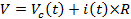 (Equation 1)
At the beginning (t = 0, immediately after the voltage supply is switched on with output V), the capacitor has not had the chance to develop any voltage, and therefore VC(t = 0) = 0, and (according to Equation 1), i(t = 0) = V/R. As time proceeds, charges build up on the capacitor and Vc will increase, and thus i(t) will decrease. Furthermore, these charges tend to repel additional charges arriving at the capacitor (i.e., opposing the charging process). After a sufficient amount of time, this charging process stops, and therefore i(t→∞) = 0 and Vc(t→) = V. This means that the capacitor is now fully charged (or has the full voltage V from the voltage source dropping across it), no more current flows, and the capacitor behaves as an open switch in this fully charged, steady state. In general, a capacitor conducts more for higher frequency or transient current, while it conducts less or not at all for lower frequency or steady state (DC) current.
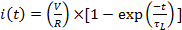
The full, quantitative time-dependent current i(t) can be solved by:
 (Equation 2)
where,
 (Equation 3)
is known as the "RC time constant" for the "RC" circuit, and characterizes in general the time scale for the response of the RC circuit (here the change in the current) upon a transient change in an input (here the switching on of the voltage supply). Such a time dependent current as given by Equation 2 is depicted in Figure 1.
In this case, the RC time also represents the characteristic time scale for charging the capacitor. It is the time scale for discharging a capacitor, namely, if a fully charged capacitor (with voltage V) is directly connected to a resistor to form a closed circuit (corresponding to replacing the voltage supply in Figure 1 by a short wire), then the current flowing through the resistor will again follow Equation 2.
An analogous analysis can be made for a resistor in series of an inductor, or an "RL" circuit such as the one shown in Figure 2. However, the behavior of an inductor is opposite to that of a capacitor, in the sense that the inductor conducts better at lower frequency (for steady state current the inductor acts as a short wire with little resistance), but conducts much less at higher frequency or in a transient situation (because an inductor always tries to oppose the change in its current). As a result, the current i(t) that would flow in the RL circuit shown in Figure 2 after closing the switch at time t = 0 (or switching on the voltage supply to output of V) would be:
 (Equation 4)
where,
 (Equation 5)
which is the general characteristic time scale for the response (here the change in current) of the RL circuit upon a transient change in an input (here the switching on of the voltage supply). Note here, i(t = 0) = 0, because initially the current through the inductor (which is the same current through the resistor) has not had a chance to change from its initial zero value (before the voltage supply is switched on), and the inductor tries to oppose any sudden change in its current. After the circuit reaches its steady state, the current is no longer changing with time, then the inductor behaves as a short wire, and indeed i(t→∞) = V/R according to Equation 4. This behavior (the current increases from 0 and approaches V/R exponentially) is depicted in Figure 2, and note it is opposite from the behavior for the RC circuit (Equation 2 and Figure 1, where the current decreases from V/R and decays to 0 exponentially).
The exponential time dependence in the RC or RL circuit is related to the dissipative nature of the resistor. In contrast, an "LC" circuit where a capacitor is directly connected to an inductor with negligible resistances, such as the one shown in Figure 3a, would exhibit an oscillatory or "resonant" behavior. Figure 3a depicts a capacitor, initially charged to have a voltage drop V, connected to an inductor (with no current through it initially) at time t = 0. One can show that the subsequent voltage on the capacitor (same on the inductor) would have the following oscillatory (sinusoidal) time dependence:
 (Equation 6)
where,
 (Equation 7)
is the "oscillation frequency" or "resonant frequency" (here, frequency refers to the angular frequency) of the LC circuit. The current through the inductor is:
 (Equation 8)
The capacitor first discharges through the inductor (VC(t) decreases and i(t) increases). When ωt reaches π/2, the capacitor is fully discharged (VC = 0) and the maximum current flows in the inductor. Then the capacitor is charged again (by the current flowing in the inductor) into the reverse polarity (VC(t) reaches -V when ωt reaches π), and then discharges again (fully discharged when ωt reaches 3π/2) and recharges to the original polarity of VC = V when ωt reaches 2π. The cycle repeats itself with the period in time (t) of,

Such an oscillatory behavior, depicted in Figure 3b, also corresponds to the capacitor and inductor swapping electromagnetic energy between each other (a capacitor stores energy in the electric field due to the voltage drop, and an inductor stores energy in the magnetic field due to the current). In the ideal situation of no resistance (and thus no dissipation) in the circuit, the oscillation can go on indefinitely. In the presence of some resistance (dissipation), for example in the circuit shown in Figure 3c, also known as an "RLC" circuit, such an oscillation will be damped (if there is no external power supply), depicted in Figure 3d, and after a sufficient amount of time both the voltage and current would reach zero.
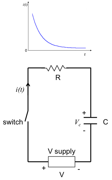
Figure 1: Diagram showing an RC circuit, with a resistor (R) in series with a capacitor (C), connected to a voltage supply with a switch. A representative time dependent current (given by Equation 2) is depicted above the figure.

Figure 2: Diagram showing an RL circuit, with a resistor (R) in series with an inductor (L), connected to a voltage supply with a switch. A representative time dependent current (given by Equation 4) is depicted above the figure.
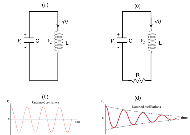
Figure 3: (a) Diagram showing an LC circuit, with an inductor (L) connected with a capacitor (C) in a closed circuit. (b) A representative time dependent voltage on the capacitor, showing undamped oscillation (given by Equation 6). (c) Diagram showing an LC circuit with a series resistance (R), also known as a RLC circuit. (d) A representative time dependent voltage on the capacitor for the circuit shown in (c), showing a damped oscillation.
Procedure
1. Using an Oscilloscope
- Obtain an oscilloscope, a small light bulb (with resistance R of a few Ω), a switch, and a DC voltage supply (or alternatively a 1.5 V battery).
- Connect the circuit as shown in Figure 4, with the switch open. The connections in this experiment can be made with cables, clamps, or banana plugs into receiving ports on the instruments.
- Select the vertical scale of the oscilloscope to a range that is close to 1 V. Select the time scale of the oscilloscope to a range that is close to 1 s.
- Close the switch (thus switching on the light bulb). Observe the light bulb as well as the trace ("waveform") on the oscilloscope screen. The oscilloscope, connected in parallel to the light bulb, will measure the voltage across the light bulb, and this voltage is proportional to the current through the light bulb.
- Now open the switch again (thus switching off the light bulb). Again observe the light bulb as well as the trace ("waveform") on the oscilloscope screen.
- Repeat the steps 1.4 and 1.5, if necessary.
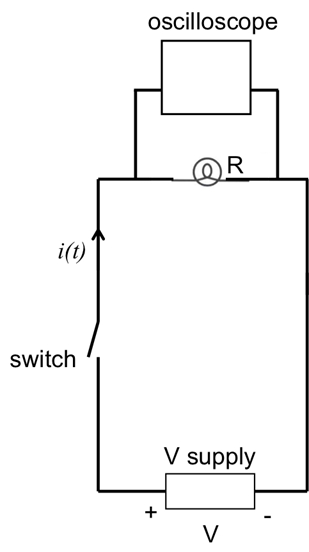
Figure 4: Diagram showing a light bulb connected to a voltage supply with a switch. An oscilloscope is connected in parallel with the light bulb to measure its voltage (proportional to the current).
2. RL Circuit
- Obtain an inductor with inductance L of 1 milliHenry (mH).
- Connect the inductor in series to the light bulb (with the oscilloscope connected in parallel to the light bulb), and to the voltage supply with an open switch, as shown in Figure 5a.
- Close the switch. Observe the light bulb as well as the waveform on the oscilloscope.
- Open the switch. Obtain another light bulb (of the same kind as the first light bulb) and connect it in parallel with the first light bulb, as shown in Figure 5b.
- Repeat step 2.3 (close the switch), and observe the light bulbs and oscilloscope.
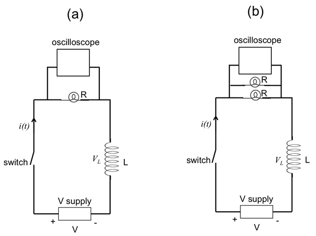
Figure 5: Diagram showing an RL circuit, with one light bulb ( a) or two parallel light bulbs ( b) acting as the resistor (R). An oscilloscope is connected in parallel with the light bulb(s) to measure the voltage across the light bulb(s), proportional to the total current.
3. RC Circuit
- Obtain a capacitor with capacitance of 1 Farad (F).
- Connect the capacitor in series with the light bulb (which is connected in parallel to the oscilloscope), and together to the voltage supply with the open switch, as shown in Figure 6a. This corresponds to the similar circuit shown in Figure 5a connected in step 2.2, except with the inductor replaced by the capacitor.
- Close the switch. Observe the light bulb as well as the waveform on the oscilloscope.
- Open the switch. Connect the second light bulb in parallel with the first light bulb, as shown in Figure 6b.
- Repeat step 3.3 (close the switch), and observe the light bulbs and oscilloscope.
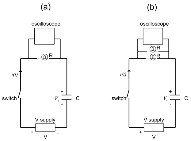
Figure 6: Diagram showing a RC circuit, with one light bulb ( a) or two parallel light bulbs ( b) acting as the resistor (R). An oscilloscope is connected in parallel with the light bulb(s) to measure the voltage across the light bulb(s), proportional to the total current.
3. LC Circuit
- Connect an 8 mH inductor in series with another open switch (switch #2) and together in parallel to a 10 µF capacitor, as shown in Figure 7. Close the switch #1 to have the capacitor charged. No light bulbs are used in this part of experiment.
- Connect the oscilloscope in parallel with the capacitor, as shown in Figure 7.
- Now open switch #1, then right away also close switch #2. Observe the oscilloscope.
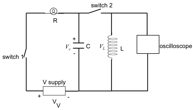
Figure 7: Diagram showing an inductor (L) with a switch connected in parallel to a capacitor (C), which is part of a series RC circuit studied in Figure 6. The oscilloscope is now connected in parallel to the inductor to measure its voltage.
Results
For step 1, the light bulb will "instantly" turn on and off when closing (step 1.4) and opening (in step 1.5) the switch. Representative oscilloscope traces are shown in Figure 8.
For step 2.3, after closing the switch, it can be observed that it takes a small but noticeable amount of time for the light bulb to turn on (instead of instantly as in step 1). When two parallel light bulbs are used (step 2.5), it takes a longer time for the light bulbs to turn on compared to the previous case (step 2.3). This is because the two parallel light bulbs give a smaller resistance (R), and thus a longer time constant τL = L/R for an RL circuit (note that the time constant may not be exactly twice as long because the two light bulbs may not have exactly the same resistances, and there may be other non-negligible resistances in the circuit). Representative traces on the oscilloscope for the two cases are shown in Figure 9. The "turning on" time scale measured on the oscilloscope is ~ ms and is consistent with the expected time constant τL based on the values of inductance and light bulb resistance.
For step 3.3, after closing the switch, it can be observed that the light bulb will glow briefly before dying out. When two parallel light bulbs are used (step 3.5), it takes a shorter time for the light bulbs to die out compared to the previous case (step 3.3). This is because the two parallel light bulbs give a smaller resistance (R), and thus a shorter RC time constant τ = RC. Representative traces on the oscilloscope for the two cases are shown in Figure 10. The "turning on" time scale of ~1 s is consistent with the expected time constant τ based on the values of capacitance and light bulb resistance.
For step 4.3, an oscillatory voltage such as those depicted in Figure 3b, 3d can be observed on the oscilloscope. Some damping of the oscillation may be observed due to the finite resistance of the wires connecting the circuit. The period of the oscillation, on the order of millisecond, is consistent with the expected LC oscillation period (2π ) based on the values of capacitance and resistance.
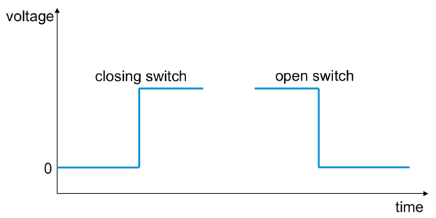
Figure 8: Representative oscilloscope traces (or "waveforms") that may be observed in the experiment depicted in Figure 4, when the switch is closed or opened, measuring the voltage across a light bulb directly connected to a voltage supply.
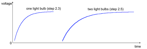
Figure 9: Representative oscilloscope traces (or "waveforms") that may be observed when the switch is closed in the experiment depicted in Figure 5, measuring the voltage across a light bulb connected in series of an inductor and a voltage supply.

Figure 10: Representative oscilloscope traces (or "waveforms") that may be observed when the switch is closed in the experiment depicted in Figure 6, measuring the voltage across a light bulb connected in series of a capacitor and a voltage supply
Application and Summary
In this experiment, we have demonstrated the time dependent response (exponential turning on and off) in RC or RL circuits, and how changing the resistance affects the time constant. We also demonstrated the oscillatory response in an LC circuit.
RC, RL and LC circuits are essential building blocks in many circuit applications. For example, RC and RL circuits are commonly used as filters (taking advantage of the fact that capacitors tend to pass high frequency signals but block low frequency signals, while the opposite is true for inductors). They are also useful for electrical signal processing, for example, taking the derivative or integral of an electrical signal. The LC circuit is a simple example of an electrical "oscillator" or resonance circuit and is a common component in circuits used for amplifiers, radio tuning, etc.
The author of the experiment acknowledges the assistance of Gary Hudson for material preparation and Chuanhsun Li for demonstrating the steps in the video.
Skip to...
Videos from this collection:

Now Playing
RC/RL/LC Circuits
Physics II
142.7K Views

Electric Fields
Physics II
77.4K Views

Electric Potential
Physics II
104.4K Views

Magnetic Fields
Physics II
33.4K Views

Electric Charge in a Magnetic Field
Physics II
33.7K Views

Investigation Ohm's Law for Ohmic and Nonohmic Conductors
Physics II
26.2K Views

Series and Parallel Resistors
Physics II
33.1K Views

Capacitance
Physics II
43.7K Views

Inductance
Physics II
21.5K Views

Semiconductors
Physics II
29.7K Views

Photoelectric Effect
Physics II
32.6K Views

Reflection and Refraction
Physics II
35.9K Views

Interference and Diffraction
Physics II
90.9K Views

Standing Waves
Physics II
49.7K Views

Sound Waves and Doppler Shift
Physics II
23.4K Views
Copyright © 2025 MyJoVE Corporation. All rights reserved