
Jet Impinging on an Inclined Plate
Overview
Source: Ricardo Mejia-Alvarez and Hussam Hikmat Jabbar, Department of Mechanical Engineering, Michigan State University, East Lansing, MI
The goal of this experiment is to demonstrate how a fluid flow exerts forces on structures by conversion of dynamic pressure into static pressure. To this end, we will make a plane jet impinge on a flat plate and will measure the resulting pressure distribution along the plate. The resultant force will be estimated by integrating the product between the pressure distribution and appropriately defined area differentials along the surface of the plate. This experiment will be repeated for two angles of inclination of the plate with respect to the direction of the jet and two flow rates. Each configuration produces a different pressure distribution along the plate, which is the result of different levels of conversion of dynamic pressure into static pressure at the plate's surface.
For this experiment, pressure will be measured with a diaphragm pressure transducer connected to a scanning valve. The plate itself has small perforations called pressure taps that connect to the scanning valve through hoses. The scanning valve sends the pressure from these taps to the pressure transducer one at a time. The pressure induces mechanical deflection on the diaphragm that the pressure transducer converts into voltage. This voltage is proportional to the pressure difference between the two sides of the diaphragm.
Principles
In steady incompressible flows with negligible changes in gravitational potential, Bernoulli's equation could be interpreted as the addition of two forms of energy: kinetic energy and pressure potential energy. In an inviscid process, these forms of energy are free to transform into each other along streamlines while keeping the initial total amount of energy constant. This energy total is called the Bernoulli's constant. For convenience, Bernoulli's equation can be expressed in dimensions of pressure using the principle of dimensional homogeneity [3]. Under this dimensional transformation, the term associated to kinetic energy is dubbed "dynamic pressure", the term associated with the pressure potential energy is called "static pressure", and the Bernoulli's constant is named "stagnation pressure". The latter can be interpreted as the maximum pressure that the flow would reach if brought to a halt by transforming all its dynamic pressure into static pressure. These principles can be better described by the following form of Bernoulli's equation:
 (1)
(1)
Where  is the static pressure,
  is the dynamic pressure, and
  is the stagnation pressure. Figure 1(A) shows a schematic of the current experiment. As shown, an air jet exits from a higher-pressure plenum through a slit of width W and span L to an enclosed space at a lower pressure named receiver. The receiver is a small room that serves as the test section for the experiment. It houses the data acquisition equipment and the experimentalists. After flowing for some distance, the jet impinges on a flat plate inside the receiver that makes an angle with the jet axis. The jet in figure 1(A) is outlined by three streamlines. The intermediate streamline divides the jet in two regions, one that gets deflected upwards and one that gets deflected downwards. Since the dividing streamline does not get deflected, it stops right at the wall at what is known as the stagnation point. At that point, all the dynamic pressure gets converted into static pressure and the pressure reaches its maximum level, . The pressure level decreases away from the stagnation point because progressively less dynamic pressure gets converted into static pressure.
Depending on the impingement angle ( in figure 1), the stagnation streamline follows a different path. When
  , the centerline of the jet is also the stagnation streamline. As is decreased, the stagnation streamline moves away from the centerline of the jet, toward trajectories that start closer to the outer edge of the jet. Since 90o is also the trajectory of maximum velocity, ergo maximum dynamic pressure, its resulting stagnation point will reach the maximum value of pressure compared to other trajectories at smaller values of . In summary, the effect of the impingement angle on the pressure profile is to reduce its maximum value and displace its peak toward regions of the plate closer to the jet exit.
The dashed line in figure 1(A) represents the net pressure distribution along the surface of the plate exposed to the jet. Note from figure 1(B) that the total pressure on the plate,  , is the addition of the surrounding pressure,
  , plus the impingement pressure or overpressure,
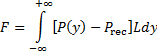
  . Since the surrounding pressure is homogeneously distributed, it cancels out and the load on the plate is strictly the result of the overpressure. This pressure distribution will be determined experimentally and used to estimate the net load on the plate according to the following integral:
 (2)
(2)
Since the experimental data is discrete, this integral can be estimated using the trapezoidal rule or the Simpson's rule [4].
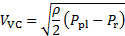
In addition, when fluids are discharged from a higher-pressure region to a lower pressure region through orifices or slits, the issuing jet tends to converge initially into a region called the vena contracta (see Figure 1 for reference) and then diverge thereafter as it flows away from the discharge port [5]. The vena contracta is in fact the first location after a jet leaves its discharge port in which the streamlines become parallel. Consequently, this is the first place along the jet in which the static pressure equals the pressure of the surroundings [5]. In the present experiment, the plenum is the higher-pressure region and the receiver is the lower-pressure region. Further, the velocity inside the plenum is negligible, and it can be considered stagnant with very good approximation. Hence, equation (1) could be used to determine the velocity at the vena contracta as follows:
 (3)
(3)
Here,  is the pressure difference between the plenum and receiver. In general, the contraction ratio between the slit width and the vena contracta is very approximately [5, 6, 7]:
 (4)
(4)
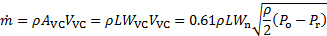
Hence, the mass flow rate can be estimated from (3) and (4) as follows:
 (5)
(5)
Here,  is the area of the vena contracta.

Figure 1. Schematic of basic configuration. A plane jet exits the plenum into the receiver through a slit of width W. The jet impinges on an inclined plate and it gets deflected while exerting a pressure load on the surface (dashed line). Please click here to view a larger version of this figure.
Procedure
1. Setting the facility
- Make sure that there is no flow in the facility.
- Set the instruments according to the schematic in figure 2.
- Adjust the plate to the desired angle . Record this value in table 1.
- Measure the jet nozzle width W. Record this value in table 1.
- Measure the plate span L. Record this value in table 1.
- Zero the pressure transducer.
- Note the calibration constant of the pressure transducer, mp (Pa/V). Record this value in table 1.
- Connect the high-pressure port of the transducer (marked as +) to the pressure tap of the plenum (marked as
 ).
). - Since all the operations take place inside the receiver, leave the low-pressure port of the transducer (marked as -) open to sense the pressure in the receiver ().
- Start the flow facility (FLL).
- Use the digital multi-meter to record the voltage
 (V) associated with the pressure difference between the plenum and the receiver sensed by the pressure transducer. Record this value in table 2.
 - Use the calibration constant mp from 1.7 to determine the pressure difference between the plenum and the receiver (
 ). Record this value on table 2.

Figure 2 . Details of data acquisition system. Schematic for equipment connections. Please click here to view a larger version of this figure.
Table 1 . Basic parameters for experimental study.
| Parameter | Value |
| Jet nozzle width (Wn) | 41.3 mm |
| Plate span (L) | 81.3 cm |
| Plate height (H) | 61cm |
| Transducer calibration constant (m_p) | 137.6832 Pa/V |
2. Running the experiment
- Connect the high-pressure port of the transducer (marked as +) to the common port of the scanning valve. Leave the low-pressure port of the transducer (marked as -) open to sense the pressure in the receiver ().
- Home the scanning valve to start your measurement from the first pressure tap position.
- Run the Traverse VI (LabView virtual instrument).
- Input the calibration constant mp in the VI.
- Set the sampling rate to 100 Hz and the total of samples to 500 (i.e. 5 seconds of data).
- Enter in the VI the position (
 ) of the pressure tap from which plate-pressure data will be acquired. Take into account that the pressure taps are spaced by 25.4mm. Hence, the position will be
  mm, where
  is the index of the tap starting at 0.
 - Record the data. The VI will read the pressure difference between the pressure tap and the receiver (
 .
. - Step the scanning valve to the next tap position.
- Repeat steps 2.6 to 2.8 until all the pressure taps are traversed.
- At the end, the VI provides a table and a plot of tap position vs pressure.
- Stop the VI.
- Change the position of the flow control plate to close the flow area roughly by half (see Figure 3 for reference). This will modify the flow rate. Use Equation (5) to determine the value of this flow rate.
- Repeat steps 2.3 to 2.11 for the new position of the flow control plate.
- Modify the angle of the impingement plate and set the flow control plate to its initial position.
- Repeat steps 2.3 to 2.14 for 80o, 70o, 60o, 50o, and 45o.

Figure 3 . Experimental setting. Test section. Left: Impingement plate in front of slit. Higher-pressure air is discharged from the plenum into the receiver through this slit. Middle: pressure taps connected to the impingement plate are distributed into the scanning valve to sample one at a time. Right: impingement plate in front of receiver discharge. The discharge has a perforated plate to regulate flow rate. Please click here to view a larger version of this figure.
3. Analysis
- For each inclination angle, plot the pressure data for both flow rates.
- Use the experimental data to estimate the force on the plate based on equation (2).
- Determine the jet velocity at the vena contracta using equation (3).
- Estimate the mass flow rate using equation (5).
Results
Figure 4 shows four sets of results obtained for the plane jet impinging on a plate at two different angles and two different flow rates. In fact, since the low-pressure side of the transducer is opened to the receiver, its readings correspond only to the overpressure , which are in fact the points shown in Figure 4.
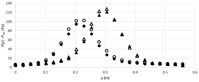
Figure 4. Representative results. Pressure distribution along the plate for two angles and two flow rates. Symbols represent:  :
:  ,
,  m/s;
m/s;  : ,
: ,  m/s;
m/s;  :
:  , m/s;
  : , m/s.
According to Figure 4, the profiles for 90o impingement are higher than the ones for 70o impingement. The reason for this behavior is that the stagnation streamline for the former case corresponds to the flow centerline, that is, the streamline for peak velocity and consequently maximum dynamic pressure. While the stagnation streamline moves away from the peak velocity line and bends away from its original path as the impingement angle decreases. This effect is sketched in Figure 1(A), and it is also the reason why the peak pressure in the pressure profile moves away from the center of the plate.
As expected, the maximum pressure decreases with flow rate (closed symbols in figure 4) because there is a general reduction in kinetic energy and hence in dynamic pressure as the flow rate decreases. This maximum pressure is in fact a measure of the stagnation pressure, , previously explained. For the case of the jet impinging the plate at 90o, this is an accurate measure of because the pressure tap coincides with the centerline, ergo the stagnation streamline, of the jet. But as suggested in figure 1a, the stagnation streamline bends away from its original path as the impingement angle decreases. Under this new condition, there is not guarantee that this streamline will exactly coincide with a pressure tap at its impingement location. Hence, the peak pressure observed at impingement angles different than 90o is just an approximation to .
Table 2 shows the results obtained in experimental measurements for two different impinging angles and flow rates.
Table 2. Representative results.
| Parameter | Run 1 | Run 2 | Run 3 | Run 4 |
| Plate angle (θ) | 90o | 90o | 70o | 70o |
| Digital multi-meter reading (E) | 2.44 V | 2.33 V | 2.44 V | 2.28 V |
| Pressure difference (P_pl-P_rec ) | 335.95 Pa | 320.80 Pa | 335.95 Pa | 313.92 Pa |
| Velocity at vena contracta (V_VC) | 10.14 m/s | 9.91 m/s | 10.14 m/s | 9.81 m/s |
| Mass flow rate ((m)) ̇ | 0.254 kg/s | 0.249 kg/s | 0.254 kg/s | 0.246 kg/s |
| Stagnation pressure (P_o ) | 127.16 Pa | 121.19 Pa | 101.78 Pa | 94.31 Pa |
| Load on the plate (F) | 16.84 N | 16.24 N | 14.11 N | 12.32 N |
Application and Summary
The experiments featured herein demonstrated the interplay of pressure and velocity to generate loads in objects by means of conversion of dynamic pressure into static pressure. These concepts were demonstrated with a plane jet impinging on a flat plate at two different angles and two different flow rates. The experiments clearly demonstrated that the load is highest at the stagnation point, where all the dynamic pressure is converted into static pressure, and its magnitude decreases as the level of conversion from dynamic to static decreases at positions away from the stagnation point. The angle of incidence has the effect of reducing the total load because it shifts the stagnation pressure from the one coinciding with the centerline (maximum) velocity to a streamline carrying lower levels of dynamic pressure.
These experiments also served the purpose of demonstrating how to determine the total load on the object exposed to the flow by numerically integrating the data obtained from pressure taps. In addition, the reverse conversion of static pressure into dynamic pressure was also used to estimate the velocity and mass flow rate of the jet. In consequence, the interplay of pressure and velocity can be used for flow diagnostics.
A concept that was not explored in the present experiment is velocimetry by Pitot - static probes. These are probes that directly measure the difference between the stagnation and static pressures, which is exactly what was used in equation (3) to determine the velocity at the vena contracta. Note that, at least in the 90o angle plate, the central pressure tap is directly exposed to the stagnation point, making it a Pitot probe. Since the pressure transducer compares the pressure of each pressure tap to the receiver's pressure, the result is a direct measurement of  . Upon substitution of this measurement in equation (3), the result is the velocity of a point on the stagnation streamline that is close to the stagnation point but still outside of its radius of influence. This measurement is of limited use in this experiment because the exact location of that point on the stagnation streamline is not known.
As mentioned before, pressure measurements can be used to determine flow velocity. In the application described herein, the change in pressure between the plenum and the receiver were enough to estimate the average velocity at the vena contracta.It was also mentioned that, incidentally, the pressure tap coinciding with the stagnation point is a Pitot tube that could be used in conjunction with a probe sensing the static pressure to determine flow velocity from equation (3) (substituting with and  with ). In fact, a single device combining a Pitot probe and a static probe, known as Prandtl tube, might be the most extended diagnostic device in fluids engineering to measure velocity. As shown in figure 5, this probe is composed by two concentric tubes. The inner tube faces the flow to detect the stagnation pressure, and the outer tube has a set of side ports that sense the static pressure. A sensor such as a pressure transducer or a liquid column manometer is used to determine the difference between these two pressures to estimate the velocity from equation (3) (again, substituting with and with ). A probe like this, or a combination of a Pitot and an independent static probe is in fact used in airplanes to determine the velocity of the wind relative to the airplane.
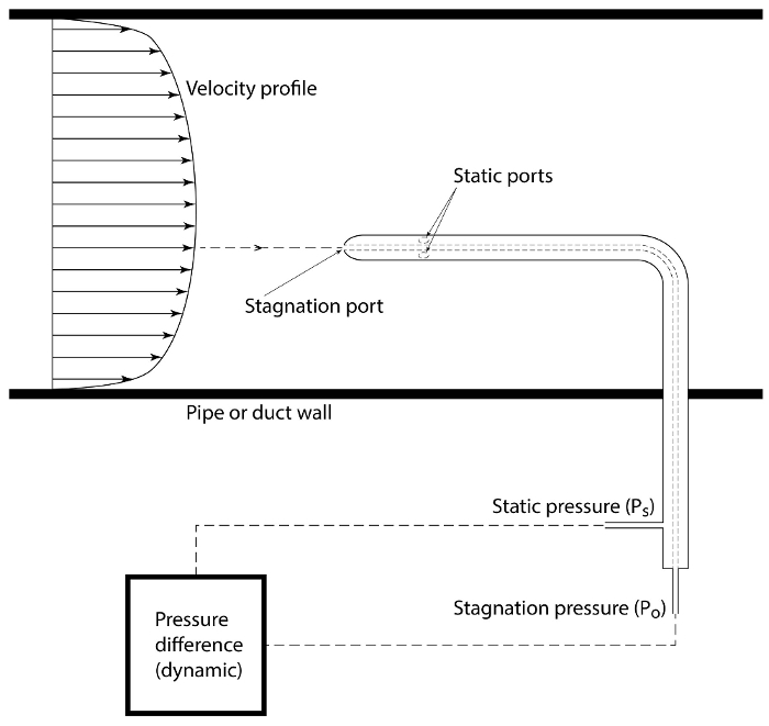
Figure 5. Flow velocimetry. Pitot-static (or Prandtl) probe to determine the velocity distribution based on the dynamic pressure. This probe is traversed across the flow field to determine the velocity at different positions. Please click here to view a larger version of this figure.
Tags
Skip to...
Videos from this collection:

Now Playing
Jet Impinging on an Inclined Plate
Mechanical Engineering
10.8K Views

Buoyancy and Drag on Immersed Bodies
Mechanical Engineering
30.2K Views

Stability of Floating Vessels
Mechanical Engineering
23.3K Views

Propulsion and Thrust
Mechanical Engineering
22.1K Views

Piping Networks and Pressure Losses
Mechanical Engineering
58.8K Views

Quenching and Boiling
Mechanical Engineering
8.2K Views

Hydraulic Jumps
Mechanical Engineering
41.3K Views

Heat Exchanger Analysis
Mechanical Engineering
28.3K Views

Introduction to Refrigeration
Mechanical Engineering
25.0K Views

Hot Wire Anemometry
Mechanical Engineering
15.9K Views

Measuring Turbulent Flows
Mechanical Engineering
13.6K Views

Visualization of Flow Past a Bluff Body
Mechanical Engineering
12.2K Views

Conservation of Energy Approach to System Analysis
Mechanical Engineering
7.4K Views

Mass Conservation and Flow Rate Measurements
Mechanical Engineering
23.0K Views

Determination of Impingement Forces on a Flat Plate with the Control Volume Method
Mechanical Engineering
26.0K Views
Copyright © 2025 MyJoVE Corporation. All rights reserved