Electric Charge in a Magnetic Field

Source: Andrew Duffy, PhD, Department of Physics, Boston University, Boston, MA

This experiment duplicates J.J. Thomson's famous experiment at the end of the 19^th century, in which he measured the charge-to-mass ratio of the electron. In combination with Robert A. Millikan's oil-drop experiment a few years later that produced a value for the charge of the electron, the experiments enabled scientists to find, for the first time, both the mass and the charge of the electron, which are key parameters for the electron.

Thomson was not able to measure the electron charge or the electron mass separately, but he was able to find their ratio. The same is true for this demonstration; although here there is the advantage of being able to look up the values for the magnitude of the charge on the electron(e) and the mass of the electron (m_e), which are now both known precisely.

 In this experiment, a beam of electrons (inside an evacuated tube) and a magnetic field are under the experimenter's control. One of the key ideas is that a magnetic field can apply a force to a moving charge. If the charge has a velocity and the magnetic field is , then the magnitude of the force is given by:

(Equation 1)

where q is the magnitude of the charge and θ is the angle between the velocity and the magnetic field. Because of the sinθ factor, the force is maximum when the velocity and magnetic field are perpendicular to one another, and there is no force when the velocity and the field are parallel to one another.

This force has a direction. The direction of the force is perpendicular to the plane defined by the velocity and the magnetic field (in other words, the force is perpendicular to both the velocity and the magnetic field). The exact direction of the force can be determined by the right-hand rule. One version of the right-hand rule is the following:

Using the right hand, point the fingers in the direction of the velocity.

Think about the component of the magnetic field that is perpendicular to the velocity (the parallel component produces no force). Keeping the fingers in the direction of the velocity, rotate the hand until the palm faces the direction of the perpendicular component of the magnetic field.

Stick out the thumb. As long as the charge is positive, the thumb should point in the direction of the force applied by the magnetic field on the moving charge.

If the charge is negative, then the force is in the opposite direction to the way the thumb points.

Because the force is perpendicular to the velocity, the force can neither speed the particle up nor slow it down. All the force can do is change the direction of the velocity. In the special case that the velocity and the magnetic field are perpendicular to one another, the result is that the charged particle follows a circular path, traveling in a circle at constant speed. This is the definition of uniform circular motion, which means Newton's second law can be applied with the acceleration as the centripetal acceleration.

In this case:

(Equation 2)

This can be rearranged to find an expression for the charge-to-mass ratio of the moving charge:

(Equation 3)

For the purposes of derivation, both sides of the equation are squared:

(Equation 4)

Which re-arranges to:

(Equation 5)

This might look like an odd thing to do, but note that in the numerator on the right-hand side, there is half the kinetic energy of the charges particle. In the experiment, the electrons gain kinetic energy, before entering the magnetic field, by being accelerated from rest through a potential difference, V. Applying energy-conservation ideas:

so,    

(Equation 6)

Inserting that into the charge-to-mass equation results in:

(Equation 7)

So in the experiment, the charge-to-mass ratio can be found by simply knowing three pieces of information, namely the accelerating voltage, the strength of the magnetic field, and the radius of the circular path followed by the charged particles.

The accelerating voltage V is set with a slider on the high-voltage power supply, with a meter that can be used to read the voltage.

The magnetic field B is produced by current running through a pair of coils, with one coil on each side of the tube. The current I is read by a digital ammeter, and the particular coils used create a magnetic field of:

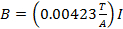(Equation 8)

The radius of the path of the beam can be found from a two-dimensional X-Y scale inside the tube (Figure 1). The current in the coils is adjusted until the electron beam passes through point G, which has coordinates of (X, Y). The X and Y values can be read easily off the scale inside the tube. Then, in the right-angled triangle shown in Figure 1, side OE has a length of R-Y, and side EG has a length of X. Applying the Pythagorean Theorem results in

(Equation 9)

Solving this equation for R results in:

  (Equation 10)

This is all the information needed to determine the charge-to-mass ratio.

Figure 1: Diagram of the geometry for the electron beam. The electrons, traveling left to right, enter the magnetic field at point F = (0, 0) and are then deflected by a magnetic field into a circular path that passes through point G = (X, Y). The adjustable magnetic field is created by two coils (known as Helmholtz coils), one on either side of the tube. The direction of the magnetic field in this picture is out of the page, but the field can be reversed so that the beam bends up, instead of down. The center of the circular path is at point O. A right-angled triangle is shown, from which the radius R can be determined.

1. Compensating for Earth's Magnetic Field

1. Note that there are two independent circuits in this experiment:
   1. Supply current to the coils that create the magnetic field ( Figure 2). The current is set by a rotary dial, and the circuit includes a digital ammeter that allows the current to be measured. A double-pole double-throw switch is used to reverse the direction of the current supplied to the coils, which reverses the magnetic field.
   2. The second circuit ( Figure 3) runs the electron tube. There is a high-voltage supply, which sets the accelerating voltage and an alternating signal of 6.3 V connected to a filament. Electrons are, in some sense, boiled off the filament and then accelerated by the accelerating voltage.
2. In the second circuit, turn on the high-voltage power supply to turn on the filament. The light that switches on inside the tube is the glowing filament.
3. Gradually turn up the high voltage to about 2,000 V. The part of the screen inside the tube, which is being hit by the electron beam, should glow blue, making the electron beam visible.
   1. Note that this does not mean electrons are blue - the coating on the screen is phosphorescent and gives off a blue glow when the atoms of this coating are energized by the electrons.
4. Adjust the current through the coils, which create the uniform magnetic field. As the current is adjusted up or down, the path of the beam changes. Adjust the current to pass the beam through a particular (X, Y) point on the grid. Make note of the magnitude of the current required to have the beam pass through that point.
5. Reverse the current to curve the beam in the opposite direction, and adjust the current until the beam passes through the point (X, −Y) (the mirror image of the original point). Again, make note of the magnitude of the current required to have the beam pass through that particular point.
6. Check to see if the magnitudes of the two currents are different. Unless the tube happens to be aligned so the electron beam is parallel to Earth's magnetic field, the Earth's field adds to the field of the coils when the current is in one direction and subtracts from it when the current is in the other direction.
7. Throughout the experiment, average the magnitudes of the two currents, the current required to have the beam pass through a particular (X, Y) point on the grid, and the current required to pass through the mirror-image point (X, −Y), to remove the effect of Earth's magnetic field.

Figure 2: Circuit diagram for the Helmholtz coils. The strength of the magnetic field created by the Helmholtz coils is proportional to the current passing through them. The current supplied to the coils by the adjustable power supply is measured by the digital ammeter. The purpose of the double switch is to easily reverse the direction of the current passing through the coils, which reverses the direction of the magnetic field. Note that the two connections to each coil are marked A and Z, and the two Z's should be connected together to ensure that the coils are producing magnetic fields in the same direction, and not in opposite directions.

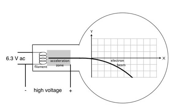
Figure 3: Circuit diagram for running the electron tube. The glowing filament that is the source of the electrons is run by a 6.3 V alternating current source. Note that the negative side of the high voltage signal is also connected to one side of the filament, while the positive high voltage signal (on the order of 2,000-3,000 V DC) is connected to an electrode on the right side of the acceleration zone. This produces a large electric field directed left in the acceleration zone, accelerating the electrons from left to right.

2. Data Collection for a Particular (X, Y) and (X, − Y) Combination

1. Note that the tubes are expensive and somewhat fragile. Do not exceed 3,500 V for the accelerating voltage, and turn the accelerating voltage down to zero when measurements are not being taken.
2. In this part of the experiment, record five sets of data, each with a different accelerating voltage with the same (X, Y) and (X, −Y) combination.
3. Note that as the accelerating voltage increases and the electrons travel faster, they do not bend as much, and thus, the magnetic field from the coils needs to be increased to have the beam pass through the same point on the screen. Choose a particular (X, Y) and (X, −Y) point to use for this part of the experiment. Use Equation 10 to calculate the corresponding radius of the beam's path.
4. For a particular accelerating voltage, record the magnitude of the current needed to have the beam pass through the chosen (X, Y) point. Reverse the current, and record the magnitude of the current needed to have the beam pass through the mirror-image point (X, −Y).
5. Average the two currents to remove the influence of Earth's magnetic field.
6. Use the average current in Equation 8 to calculate the strength of the magnetic field.
7. Use the values of the accelerating voltage, radius, and magnetic field to calculate the magnitude of the charge-to-mass ratio of the electron.
8. Choose a new accelerating voltage, and repeat steps 2.3-2.7. Continue to do this until five sets of data have been collected.
9. Compute the magnitude of the average charge-to-mass ratio for the electron.

3. Data Collection for a Particular Accelerating Voltage

1. Collect five more data sets. This time, keep the accelerating voltage constant and change the (X, Y) and (X, −Y) points that the beam passes through. Record the data.
2. Compute the magnitude of the average charge-to-mass ratio for the electron.
3. Average the two average charge-to-mass ratios determined from Section 2 and 3, and state possible sources of error in the experiment.

Representative results for Section 2 can be seen in Table 1. Those values give an average charge-to-mass ratio of 1.717 x 10^-11 C/kg. Note that that is the magnitude of the ratio, because the charge of the electron is a negative value.

Representative results for Section 3 can be seen in Table 1. Those values give an average charge-to-mass ratio of 1.677 x 10^-11 C/kg. Again, this is the magnitude of the ratio, because the charge of the electron is a negative value.

Averaging out the two values of the magnitude of the charge-to-mass ratio and rounding to three significant figures gives a value of 1.70 x 10^-11 C/kg.

This ratio is known rather precisely, seeing as the value of the charge of the electron and the mass of the electron of many significant figures is known. Using these known quantities, it can be determined that the magnitude of the charge-to-mass ratio is:

1.7588047 ± 0.0000049 C/kg

Note that the experimentally determined value is about 4% lower than this. In fact, all ten of the values are lower than the accepted value, which is an indication of a systematic error. The most likely source of such a systematic error would be in one of the meters, particularly in the meter that gives the value of the high voltage. If that meter gave readings that were consistently slightly lower than the actual value, it could explain the slightly low charge-to-mass ratio values all by itself.

The presence of Earth's magnetic field is not a source of error, because the experiment corrected for the effect of Earth's field by averaging the two current values. However, one of the assumptions in deriving the equation was that the magnetic field produced by the coils is uniform. The field is uniform inside an infinitely long solenoid, but is not perfectly uniform in the region inside the two finite coils used in this experiment, so that could be a possible source of error.

X = 7 cm    Y = 1 cm    R = 25 cm

Accelerating voltage (V)	Magnitude of current to pass through (X, Y)	Magnitude of current to pass through (X, −Y)	Average current (A)	Magnetic field (T)	e/m ratio (C/kg) x 1011
1,800	0.1537	0.1205	0.1371	0.0005799	1.713
2,000	0.1615	0.1242	0.14285	0.0006043	1.753
2,500	0.1800	0.1426	0.1613	0.0006823	1.718
3,000	0.1993	0.1571	0.1782	0.0007538	1.690
3,500	0.2136	0.1694	0.1915	0.0008100	1.707

Table 1: A filled-in table of the data collection for a particular (X, Y) and (X, −Y) combination.

Accelerating voltage = 2,700 V

X (cm)	Y (cm)	R (cm)	Magnitude of current to pass through (X,Y)	Magnitude of current to pass through (X,-Y)	Average current (A)	Magnetic field (T)	e/m ratio (C/kg) x 1011
7	1	25	0.1875	0.1500	0.16875	0.0007138	1.696
8	2	17	0.2702	0.2270	0.2486	0.001052	1.690
7	2	13.25	0.3378	0.2953	0.31655	0.001339	1.716
9	2	21.25	0.2166	0.1826	0.1996	0.0008443	1.678
10	1	50.5	0.1006	0.0710	0.0858	0.0003629	1.608

Table 2: A filled-in table of the data collection for a particular accelerating voltage.

This experiment, first performed by J.J. Thomson in the late 19^th century, demonstrated the existence of the electron, making it a tremendously important experiment from a historical perspective. Electrons have since been exploited in countless electronic devices.

The following is a list of some applications of charged particles that are traveling in circular or spiral paths, and thus they are traveling in a magnetic field:

1)The formation of the Northern Lights (Aurora Borealis) and Southern Lights (Aurora Australis) by charged particles that spiral around the magnetic field lines of the earth and deposit their energy in the polar regions.

2)A cathode-ray tube, which used to be the basis for all televisions, before the newer technologies of LCD, LED, and plasma screens.

3)A mass spectrometer. Some mass spectrometers separate ions based on their mass by bending their trajectories into circular paths using a magnetic field. The radius of the path followed by a particular ion is proportional to its mass.

4)The Large Hadron Collider (LHC), which is the famous 27 km circumference instrument buried underground along the France-Switzerland border, where physicists recently performed experiments to prove the existence of the Higgs boson, which is responsible for why particles have mass.