Method of Standard Addition

Source: Laboratory of Dr. Paul Bower - Purdue University

The method of standard additions is a quantitative analysis method, which is often used when the sample of interest has multiple components that result in matrix effects, where the additional components may either reduce or enhance the analyte absorbance signal. That results in significant errors in the analysis results.

Standard additions are commonly used to eliminate matrix effects from a measurement, since it is assumed that the matrix affects all of the solutions equally. Additionally, it is used to correct for the chemical phase separations performed in the extraction process.

The method is performed by reading the experimental (in this case fluorescent) intensity of the unknown solution and then by measuring the intensity of the unknown with varying amounts of known standard added. The data are plotted as fluorescence intensity vs. the amount of the standard added (the unknown itself, with no standard added, is plotted ON the y-axis). The least squares line intersects the x-axis at the negative of the concentration of the unknown, as shown in Figure 1.

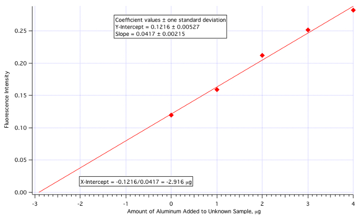
Figure 1. Graphic representation of method of standard addition.

In this experiment, the method of standard additions is demonstrated as an analytical tool. The method is a procedure for the quantitative analysis of a species without the generation of a typical calibration curve. Standard addition analysis is accomplished by measuring spectroscopic intensity before and after the addition of precise aliquots of a known standard solution of the analyte.

This experiment studies non-fluorescent species by reacting them in such a way as to form a fluorescent complex. This approach is commonly used in the investigation of metal ions. Aluminum ions (Al³⁺) will be determined by forming a complex with 8-hydroxyquinoline (8HQ). The Al³⁺ is precipitated by 8HQ from aqueous solution and then is extracted into chloroform; the fluorescence of the chloroform solution is measured and related to the concentration of the original Al³⁺ solution. Sensitivity in the part-per-million (ppm or μg/mL) range is expected for this experiment.

The reaction is

The amount of aluminum in each sample during this experiment is calculated as follows:

Blank	0
Unknown + 0 mL Standard	VUnknown(CUnknown) = 25 mL(CUnknown)
Unknown + 1 mL Standard	VUnknown(CUnknown) + VStandard(CStandard) = 25 mL(CUnknown) + 1 mL(1 μg/mL)
Unknown + 2 mL Standard	VUnknown(CUnknown) + VStandard(CStandard) = 25 mL(CUnknown) + 2 mL(1 μg/mL)
Unknown + 3 mL Standard	VUnknown(CUnknown) + VStandard(CStandard) = 25 mL(CUnknown) + 3 mL(1 μg/mL)
Unknown + 4 mL Standard	VUnknown(CUnknown) + VStandard(CStandard) = 25 mL(CUnknown) + 4 mL(1 μg/mL)

1. Preparing the Reagents

1. 100 ppm standard Al³⁺ solution: Dissolve 0.9151 g aluminum nitrate (Al(NO₃)₃•9H₂O) into a 1-L volumetric flask with DI water.
2. 8HQ solution in 1 M acetic acid (2% wt/vol): Add 2.0 g of 8-hydroxyquinoline to a 100-mL volumetric flask.
3. Carefully add 5.74 mL glacial acetic acid to the 100-mL flask, then dilute to the mark with DI water. This allows the 8-hydroxyquinoline to dissolve in aqueous phase.
4. 1 M NH₄⁺/NH₃ buffer (pH~8): Add 20 g of ammonium acetate (NH₄OAc) to a 100-mL bottle.
5. Add 7 mL of 30% ammonium hydroxide to this 100-mL bottle, and dilute to the mark with DI water. This helps neutralize the acid in the 8HQ solution when combined.
6. Other reagents include anhydrous sodium sulfate (Na₂SO₄) and chloroform (Spec grade).

2. Preparing the Samples

1. Prepare a 1.00 ppm standard Al³⁺ solution by adding 1.0 mL of the 100-ppm stock Al³⁺ solution with a pipette to a 100-mL volumetric flask.
2. Place six 125-mL separatory funnels onto the rings that are on a large ring stand located in the hood. They should be labeled as follows: BL, 0, 1, 2, 3, 4. Make sure all glassware is scrupulously clean, as it is difficult to obtain quantitative results if little beads of chloroform stick to the walls of the glassware.
3. Add 25.00 mL of the unknown Al³⁺ solution to the five separatory funnels labeled 0, 1, 2, 3, & 4. In this example, the unknown concentration is 0.110 ppm.
4. Add 0, 1.00, 2.00, 3.00, and 4.00 mL of the 1.00-ppm standard Al³⁺ solution, respectively, to the 5 funnels with a 1-mL pipette.
5. Prepare a BLANK by adding 25.00 mL of distilled water to the separatory funnel labeled BL.
6. Add 1.0 mL of the 8-hydroxyquinoline solution with a pipette to each of the six solutions.
7. Add 3.0 mL of buffer solution with a pipette to each of the six solutions.
8. Extract each solution twice with 10 mL of chloroform, shaking vigorously for 1 min each time. Remember to occasionally vent the separatory funnel to release pressure buildup. (NOTE: A good extraction only takes place when there is a lot of liquid-liquid contact between the phases).
9. Collect the chloroform in a clean, dry 100-mL labeled beaker. Chloroform has a density of close to 1.5 g/cm³, so it is the lower layer. There should be no trace of yellow color left in the aqueous phase after a complete extraction.
10. Transfer the combined chloroform extract from each beaker into their respective 25-mL volumetric flask and dilute to the mark with chloroform. Be sure to place stoppers in each volumetric flask to keep any chloroform from evaporating.
11. Add ~1 g of anhydrous sodium sulfate (Na₂SO₄) to each of the six 100-mL beakers from step 2.9. The sodium sulfate helps remove any trace of water that may be present in the chloroform extract.
12. Transfer the solutions back to their respected beakers. Swirl carefully to facilitate dehydration of any water in the sample.
13. Decant the chloroform extracts into a quartz fluorimeter cell (Note: Chloroform will dissolve a plastic polystyrene cell).

3. Selecting the Excitation Wavelength

Determine the excitation and emission wavelengths by running scans, then simply read and record the fluorescence intensity of all samples at those values. The excitation and emission bandwidths are preset at 5 nm. The complex absorbs in the near UV, so the excitation wavelength should be about 385 nm. Initially, monitor the fluorescence at 500 nm in the emission branch.

1. On the Fluorimeter, verify that both the internal and outer cooling fans in the fluorimeter are turned on prior to powering up the xenon lamp. The xenon lamp gets very hot, and requires continual cooling.
2. Turn on the high voltage (HV) to the PMT detector to 400 V.
3. Open both of the shutters.
4. Open the data acquisition program on the computer, here it's "100nmFluorScan".
5. Place the "Sample + 2 mL added" (2) solution into the quartz cell to use for determining the best excitation and emission wavelengths.
6. With the emission wavelength initially set at 500 nm, run an excitation scan from 335-435 nm with a scan speed of 2 nm/s.
7. From the resulting fluorescence plot, determine the maximum fluorescence excitation wavelength (EXλ_max), and set the instrument to that value.

4. Selecting the Emission Wavelength

1. Set the fluorimeter emission wavelength to 450 nm.
2. Set the emission wavelength range to run a 100 nm scan from 450-550 nm.
3. To start the scan, click the "start trial" button on the program at the same time of pressing the "START" button on the front panel of the fluorimeter.
4. From the resulting fluorescence plot, determine the maximum fluorescence emission wavelength (EMλ_max), and set the instrument to that value (Figure 2).

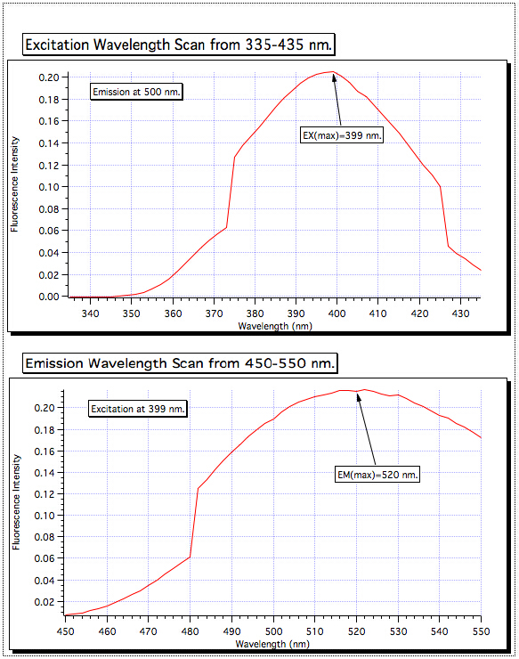
Figure 2. Determining optimum EXλ_max and EMλ_max Wavelengths.

5. Measuring the Fluorescence of the Samples

1. All samples are run at EMλ_max and EXλ_max. Scans are not needed for each sample, but just the fluorescence value at these conditions. Starting with the most dilute sample (blank), place in a quartz cell and then in instrument. Record the fluorescent intensity in lab notebook.
2. Repeat for all other samples.
3. Remember that the Blank Relative Intensity must be subtracted from the Relative Intensities of each solution prior to creating the calibration chart.

6. Creating the Standard Addition Plot

1. Plot the fluorescence intensity vs. µg of Al³⁺ added.
2. Determine the least-squares value of the resulting plot, and record both the slope and intercept.
3. Determine the µg of Al³⁺ in the unknown sample from the equation µg of Al³⁺ = -b/m
4. Knowing that the unknown aluminum had a volume of 25.0 mL added to each sample, determine the concentration of the aluminum in the unknown.

A scan of the excitation wavelength from 335–435 showed the highest absorption at 399 nm, so the excitation monochromator was set for that value. Then the emission scan was performed from 450–550 nm, and the strongest signal was found to be at 520 nm. These are the wavelengths that are used for all of the samples.

Sample	Fluorescence Intensity	Corrected Fluorescence Intensity
Blank	0.008	0.000
Sample	0.128	0.120
Sample + 1 mL	0.167	0.159
Sample + 2 mL	0.220	0.212
Sample + 3 mL	0.260	0.252
Sample + 4 mL	0.290	0.282

A plot of fluorescence (Figure 3) vs. µg of Al³⁺ added (Figure 4) yielded a least-squares line of:

Fluorescence Intensity = 0.0417 x (µg of Al³⁺ added) + 0.1216

Amount of Al³⁺ = -(Y-Int)/Slope = -0.1216/0.0417 = -2.916 µg/mL

Since the amount of unknown added was 25 mL, then the 2.916 µg/mL value needs to be divided by 25.

Unknown Aluminum Concentration = 2.916 µg/mL / 25.0 mL = 0.117 µg/mL = 0.117 ppm
which is quite close to the actual value of 0.110 ppm (6.4% error).

Figure 3. Fluorescence of the samples.

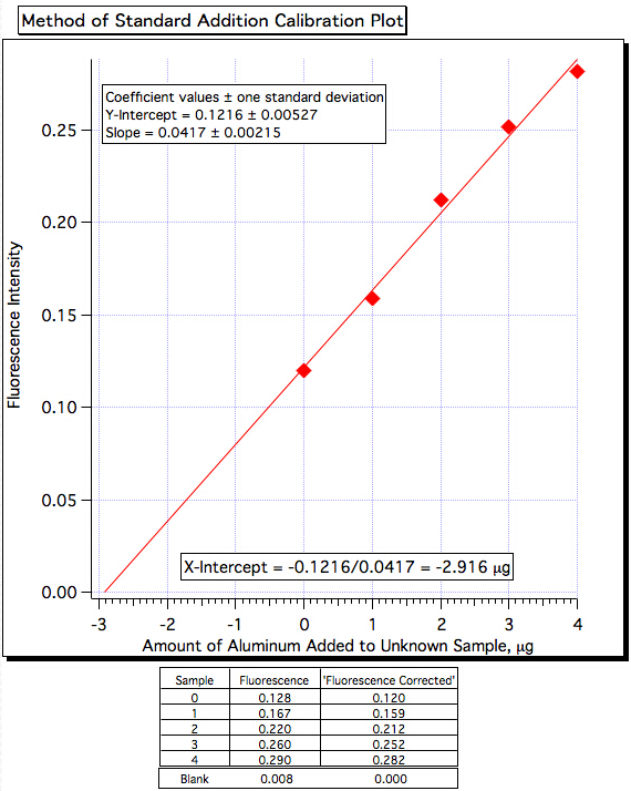
Figure 4. The standard addition calibration plot.

The method of standard additions is often the technique utilized when accurate quantitative results are desired, used in analytical analysis such as atomic absorption, fluorescence spectroscopy, ICP-OES, and gas chromatography. This is often used when there are other components in the sample of interest that causes either a reduction or enhancement of the absorbance desired for quantitative results. When this is the case, one cannot simply compare the analytes signal to standards using the traditional calibration curve approach. In fact, matrix effect evaluation should be a mandatory part of the validation procedure.

Another example where standard additions can be used is when extracting silver from old photographic waste. The waste contains silver halides, and can be extracted so the silver can be reclaimed. By spiking the unknown "waste" with known amounts of silver, this method can predict the amount of silver obtained from the photographic film.

Workers who are exposed to benzene manufacturing plants are often tested to verify they are safely below the accepted levels of benzene. Their urine is tested for the chemical, and that is the biological matrix. Also, the amount of analyte suppression varies for different people, so a single calibration kit will not work. With the method of standard addition, every employee can be tested and evaluated accurately.