
Micro-CT Imaging of a Mouse Spinal Cord
Overview
Source: Peiman Shahbeigi-Roodposhti and Sina Shahbazmohamadi, Biomedical Engineering Department, University of Connecticut, Storrs, Connecticut
It's a little-known fact that the discovery and (inadvertent) use of X-rays garnered the first ever Nobel Prize in Physics. The famous X-ray image of Dr. Röntgen's wife's hand from 1895 that sent shock waves through the scientific community looks like most modern day 2D medical X-ray images. Though it is not the newest technology, X-ray absorption imaging is an indispensable tool and can be found in the world's top R&D and university labs, hospitals, airports, among other places. Arguably the most advanced uses of X-ray absorption imaging involve attaining information like the kind found in a 2D medical X-ray but realized in 3D through a computed tomography (CT or micro-CT). By taking a series of 2D X-ray projections, advanced software is capable of reconstructing data to form a 3D volume. The 3D information can, and most likely will include information from the inside of the probed object without having to be cut open. Here, a micro-CT scan will be obtained, and the major factors impacting image quality will be discussed.
Principles
X-rays can be viewed as photons with an energy range of 0.1 - 100 keV or electromagnetic waves with wavelengths ranging from 0.01 - 10 nm. X-rays can be created in several different ways, but here the discussion is limited to continuous spectra cone-beam X-ray imaging. These X-rays are created by a phenomenon known as "Bremsstrahlung," which means "braking radiation" in German. This occurs when a charged particle undergoes an acceleration [1]. In an X-ray source, a negatively charged electron is shot in a vacuum tube and impacts a target material (usually tungsten, molybdenum, copper, or another metal) and through its deceleration, emits photons on the scale of an X-ray. A continuous spectrum of X-rays is generated because the deceleration is not uniform nor instantaneous, though there are spikes in the distribution centered around the characteristic energies of the target material as seen in [2]. There are different curves for different energies and target materials. This is a very important thing to consider when performing a micro-CT scan and will be discussed in a later section.
A typical micro-CT system features three primary components, as shown in [3]. The basic components of this system include: a) X-ray source, b) rotational stage for sample mounting, and c) flat panel or optical objective with CCD detectors. X-rays leave the source and are either absorbed, transmitted, or scattered by the sample before arriving at the detector. Absorption is the predominant interaction measured in microCT, as different materials in the body absorb X-rays differently. For example, bones contain a lot of atomic calcium, which absorbs X-rays well. Thus, bones block X-rays from reaching the detector, and end up showing up in the image as a shadow. The sample is then rotated incrementally and the process is repeated until the sample has been imaged for 360° or in some cases, 180°. The output of the tomography is a series of 2D projections at different orientations that can be reconstructed into a 3D volume.
Micro-CT is a form of microscopy, earning its name from its ability to resolve micro-scale features. The limitation of resolution for this specific category of micro-CT is governed by the source spot size and energy spread, and the detector's type and efficacy; not by the X-ray's wavelength. The best resolution possible for this category of micro-CT is around 500-700 nm in three dimensions. Though, it is possible to detect features a tenth or hundredth of that size.
Magnification is performed in most CT systems by means of geometric magnification. The image in [3] illustrates the idea of geometric magnification. It is easily imagined as a shadow effect. The closer a light source is to an object; the larger the object's shadow will appear on a wall or screen. Similarly, if that wall or screen were to move away from the stationary light source and sample, the object's shadow would increase in size but grow fainter. Optimizing the X-ray source and detector working distances is a very challenging and mentally stimulating task when sufficient signal, high resolution, and a short scan time are desired. As with anything, there are limitations on geometric magnification, where the idealization of a point source is destroyed and aberrations become overbearing.
One of the many challenges in micro-CT is that the visual quality of the 3D volume will be somewhat unknown to the investigator until the scan is finished and reconstructed. Though, with enough experience, a careful examination of a few 2D projections can provide enough information to feel confident about a CT scan. In the following sections, a set of exercises will uncover the effects of different imaging parameters on a data set and will equip a scientist with the understanding necessary to get a clean 3D volume. For the purposes of this investigation, biological samples will be probed though the procedure is not limited to a sample type.
Mounting a sample sounds like a trivial step but it is one of the most important and overlooked. Regardless of the application, the sample should be mounted in the most compact way possible. Considering the image in [3], imagine if the range of source and detector positions were limited because the sample stuck out in one direction and how that would affect geometric magnification. In addition to working distance, mounting greatly affects throughput. If the sample was an intact knee joint from a rat, it would make sense to mount the sample so that the tibia and femur stood upright. This way, the X-rays would pass through a short distance and there would be sufficient signal at the detector. The last thing to consider when mounting a sample is stability. The greatest enemy to micro-CT is movement. If the magnitude of sample movement approaches the resolution of the scan, it will probably be useless data. Movement should be limited by secure adhesion to a mount and with control to sample compositional change. For biological samples, that means ensuring that it will not change morphology through evaporation over the length of the scan. Suspension in agarose gel or wrapping in a thin layer of paraffin film are both possible approaches to avoid dehydration and movement.
X-ray energy will also have a great effect on the quality of the final 3D volume. The goal is to acquire a sufficient signal at the detector while having sufficient attenuation from the sample. X-ray attenuation follows Equation (1), where I is the final number of counts (intensity), I0 is the initial number of counts, µ is the mass absorption coefficient which is unique to a given material and X-ray energy (widely published), ρ is the material's density, and x is the X-ray path length.
 (1)
(1)
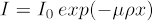
Ideally, I/I0 (a.k.a. transmission value) should be between 5 - 95% for all orientation of the sample, with the best results coming around the middle range. To check this value, take an image of the sample and then divide the image's pixel values by an image of air (i.e. with the sample outside the field of view). This normalization is commonly found in system software workflows. It is not often that biological samples demand the use of X-ray filtering at the source, so that will not be covered here. In addition to having an ideal transmission value, the ideal number of counts for any part of the sample is 5000 counts. To secure this, the exposure time per projection may need to be increased. This will increase the overall scan time. Figure 1 displays clean 2D projections.
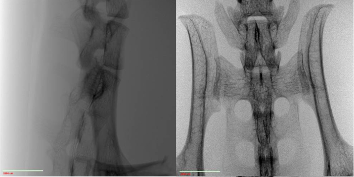
Figure 1: 2D images of mouse spinal cord normalized against air at 0° (left) and 90° (right).
Procedure
1. Mounting a Sample (Bone)
- For examining a network of bones, like a spine, suspend the structure in an agarose gel and allow to cure in a very thin-walled plastic tube (Figure 2). The thinness of the tube is very important, greatly affecting the signal throughput and overall image quality. This in turn affects your ability to resolve features. The transmission value of the tube should be as close to 100% as possible.
- Mount the tube on sample stage with tape or by making a custom stand, ultimately ensuring that the sample is stationary and stable when the stage rotates.
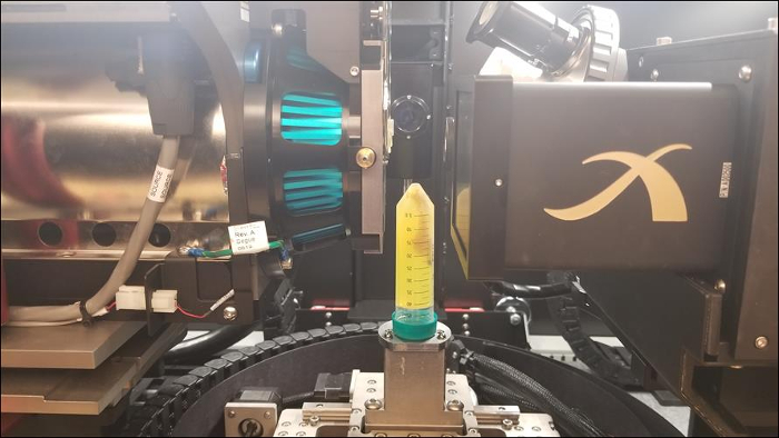
Figure 2: Mouse spine suspended in agarose gel inside thin-walled plastic tube sitting on sample stage of micro-CT system.
2. Image Acquisition
- Turn on the X-ray source to an energy around the range of 90 keV (90 kV and 10 W).
- After the source warms-up and settles on the energy, acquire an image through the system's software.
- Check the transmission value by normalizing the image against an image of air. For automatic reference acquisition and application, ensure the sample can move in a given direction without crashing.
- If image has too high of a transmission, lower the energy incrementally until the transmission value is sufficient. Be sure to increase the exposure time accordingly so that the image doesn't appear noisy and grainy. If the image has too low transmission, increase the energy incrementally until the transmission value is sufficient.
- Begin to move the X-ray source closer to the sample, while being very careful not to crash them. Bringing the source as close as possible to the sample is a step in the direction of maximizing throughput and securing the best possible resolution.
- As this is done, refine the field of view of the sample by shifting the sample stage with its linear actuators.
- The software will show a parameter known as pixel size which is treated similar to the current resolution (though it is indeed different).
- If the number is still too large and the source is very close, the detector can begin to move away from the sample.
- If the number is too small, cautiously move the detector closer to the sample.
- Try different optical objectives and detector positions as well but beware of the complication this introduces when trying to optimize the scan parameters.
- Check every orientation of the sample to ensure there are no crashes to find the best exposure time. This is performed because of the change of working distance, pixel size, and sample position.
- Slowly rotate the sample by 2-degree increments while monitoring its position relative to the source and detector via the in-cabinet camera. Be sure to move the source and detector away if a collision might occur.
- Find the longest X-ray path length that results in the lowest number of counts/transmission values and find the exposure time needed to secure about 5000 counts everywhere.
3. Tomography Submission and Reconstruction
The reconstruction process from a user perspective is not more complicated than any of the other parameter selections made in the earlier steps. However, the programming and computational expense for this process is actually quite substantial. Users must aim to best understand what is happening underneath the smooth software UI and how decisions impact the final product. Many CT systems utilize iterative algebraic reconstruction algorithms in which the 2D projections are converted into a series of linear equations describing pixel values. Some other systems utilize filtered back projection algorithms where Radon transforms convert the projections to a sinogram and are then passed through a series of line integration operations. Of course, some use other approaches and even hybrid methods. At the lowest level of involvement with these algorithms, it is known that number of projections and the total rotated displacement have an impact on the final reconstructed volume.
- First, decide whether to scan over 180° or 360° based on the aspect ratio of the sample. If the sample has a high aspect ratio such that the X-ray path length is about 4 or more times longer at the 90°-orientation than the 0°-orientation than a 180°-scan would be a smart choice. (The argument being that the information gathered on the short X-ray path length is not that different from one side to the other. If more projections can be dedicated to the long X-ray path length orientations than the data set will benefit. The angular displacement between projections will be lower and there will more information from those tricky orientations being fed into the reconstruction algorithms.) If the aspect ratio is not that high, use 360°-scans.
- Next, choose the number of projections and total angular displacement, which will dictate the angle between projections. The smaller this angle, the less interpolation will be conducted and less fine feature information will be truncated. (A balance must be established because more projections mean a longer scan time, which correlates to a larger window where samples can move, less time to scan other things, and a shorter source lifetime. A rule of thumb is to have at least 800 projections over 360° and to not exceed 3200 projections.
- Submit the scan.
- After the tomography finished (usually between 4 - 16 hours), bring 2D series of images into the system's (or some open source) reconstruction software.
- Select the optimal center shift correction. Center shift is a parameter that aligns the projects to line up (think of a roughly shuffled deck of cards that need to be collected and aligned to sit like a neat stack). This value is usually somewhere between -10 to 10 pixels.
- Select the optimal beam hardening correction coefficient. Beam hardening correction is an artificial removal of contrast produced by sample filtering. If a sample is thick enough or contains a range of light and heavy materials, it will have false contrast based on the attenuation of low-energy (soft) X-rays. This should be applied conservatively. An average value is somewhere between 0 - 0.5.
- Submit reconstruction.
Results
The following images give an overview of results that can be obtained from using micro-CT with the above stated procedure. Qualitative measurements on varying absorption can be directly noted based on these images. Quantitative data such as material porosity, feature size and distribution, etc. would require additional image processing in a different software.
Figure 3: 3D volume of mouse spinal cord (left) and two digital cross-sectional slices (right)
Application and Summary
This experiment examined the many factors that should be considered when using micro-CT, particularly for a biological sample. This project was designed to help the investigator understand how their decisions will impact the data that micro-CT can provide. As demonstrated there are many dependent and sensitive parameters that should be considered including: mounting, X-ray energy, exposure time, source and detector positioning, number of projections, and total scan angular displacement. This exercise is meant as an introduction and only scratches the surface of control over a CT data set.
This experiment focused on giving an introduction to micro-CT with respect to imaging a biological sample but the application of 3D X-ray tomography extends to the worlds of microelectronics, geology, additive manufacturing, coatings, fuel cells, and so much more. These microscopes are used for inspection, failure analysis, characterization, quality control, and even non-destructive testing. Because real, 3D information is now accessible non-destructively, the geometries extracted from CT can be imported to simulations where objects can be tested virtually.
Skip to...
Videos from this collection:

Now Playing
Micro-CT Imaging of a Mouse Spinal Cord
Biomedical Engineering
8.3K Views

Imaging Biological Samples with Optical and Confocal Microscopy
Biomedical Engineering
36.3K Views

SEM Imaging of Biological Samples
Biomedical Engineering
24.1K Views

Biodistribution of Nano-drug Carriers: Applications of SEM
Biomedical Engineering
9.6K Views

High-frequency Ultrasound Imaging of the Abdominal Aorta
Biomedical Engineering
14.8K Views

Quantitative Strain Mapping of an Abdominal Aortic Aneurysm
Biomedical Engineering
4.6K Views

Photoacoustic Tomography to Image Blood and Lipids in the Infrarenal Aorta
Biomedical Engineering
5.9K Views

Cardiac Magnetic Resonance Imaging
Biomedical Engineering
15.0K Views

Computational Fluid Dynamics Simulations of Blood Flow in a Cerebral Aneurysm
Biomedical Engineering
12.0K Views

Near-infrared Fluorescence Imaging of Abdominal Aortic Aneurysms
Biomedical Engineering
8.4K Views

Noninvasive Blood Pressure Measurement Techniques
Biomedical Engineering
12.1K Views

Acquisition and Analysis of an ECG (electrocardiography) Signal
Biomedical Engineering
107.0K Views

Tensile Strength of Resorbable Biomaterials
Biomedical Engineering
7.7K Views

Visualization of Knee Joint Degeneration after Non-invasive ACL Injury in Rats
Biomedical Engineering
8.3K Views

Combined SPECT and CT Imaging to Visualize Cardiac Functionality
Biomedical Engineering
11.2K Views
Copyright © 2025 MyJoVE Corporation. All rights reserved