Electrochemical Impedance Spectroscopy

Source: Kara Ingraham, Jared McCutchen, and Taylor D. Sparks, Department of Materials Science and Engineering, The University of Utah, Salt Lake City, UT

Electrical resistance is the ability of an electrical circuit element to resist the flow of electricity. Resistance is defined by Ohm's Law:

    (Equation 1)

Where  is the voltage and  is the current. Ohm's law is useful for determining the resistance of ideal resistors. However, many circuit elements are more complex and can't be described by resistance alone. For example, if an alternating current (AC) is used then the resistivity will often depend on the frequency of the AC signal. Instead of using resistance alone, electrical impedance is a more accurate and generalizable measure of a circuit element's ability to resist the flow of electricity.

Most commonly, the goal of electrical impedance measurements is the deconvolution of a sample's total electrical impedance into contributions from different mechanisms such as resistance, capacitance, or induction.

During Electrochemical Impedance Spectroscopy (EIS) an AC voltage is applied to a sample at different frequencies and the electrical current is measured. When dealing with AC currents impedance () replaces resistance () in Ohm's law. If the original AC signal is sinusoidal then a linear response means the current produced will also be sinusoidal, but shifted in phase. Accounting for the frequency and phase shift of the voltage and current is most easily accomplished by utilizing Euler's relationship and complex numbers where we have both a real and an imaginary component to . From this we can build equations for impedance for different components of a circuit:

1.Resistor:       (Equation 2)

2.Capacitors:      (Equation 3) 

3.Inductor:         (Equation 4)        

Where  is the frequency of the AC current,  is the capacitance,  is the inductance, and  is the imaginary unit. From these equations you can see that impedance as a resistor is independent of frequency, inversely related to frequency as a capacitor, and directly related frequency as an inductor.

A Nyquist plot is generated from the frequency response to the electrical impedance by plotting the imaginary component on the y-axis and the real component on the x-axis. The instrument applies an alternating field voltage to the sample and measures the current response. The real and imaginary components of impedance are calculated by determining the phase shift and change in amplitude at different frequencies. An example of this is shown in Figure 1. This plot is then used to build a circuit model that best represents the impedance of the sample.

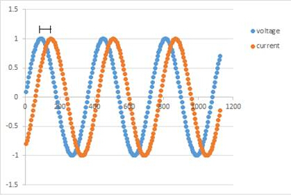
Figure 1: A representation of the phase shift between the applied voltage and the measured current.

One of the simplest Nyquist plots is that of a semi-circle which can be seen in Figure 2. The plot in Figure 2 is represented by a resistor in series followed by a resistor and capacitor in parallel-- this is known as equivalent circuit modeling. Different physical processes correspond to elements in the circuit model; for example, an electrical double layer corresponds to a capacitor. In Figure 2, a Nyquist plot is shown that is best modeled by a Randle cell. This a common starting place for the interpretation of a Nyquist plot. After the Nyquist plot is complete, the software will present you with equivalent circuit models you can choose from to model your data. If the Nyquist plot does not have a good fit from the computer-generated fits, you can build your own circuit to fit the data. However, this can be a complicated task. It is important to start simple and build up from there. It is also important to remain realistic based off what you know about the sample you are testing, to ensure that you do not build an unrealistic model. For starters, if the first point is on the real axis, it's commonly modeled as a resistor. As you move along the curve you can add or remove circuit elements to generate a better fit.

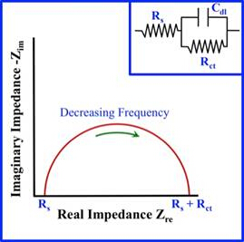
Figure 2: Image of a simple Nyquist Plot and its equivalent Randle cell model.

The concept that we plan to model in this experiment is how to test samples with EIS and use the Nyquist plot to build a model circuit which might represent the observed impedance data. For the first part of the experiment we will demonstrate how to run a control sample that produces a known circuit model that the software can easily recognize. For the second part, we can demonstrate how to test an experimental sample and again use the software to generate a model circuit the best models the electrical impedance of the sample.

1. Obtain a test module and hook it up to the EIS instruments via two electrodes. The test module, pictured in Figure 3, provides data that can be used to model a simple, known circuit. It can be used to confirm that the wires are hooked up to the machine correctly and that all the machinery parts are functioning.

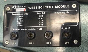
Figure 3: Test module.

2. To start flowing current through the sample, open the Zplot software on the computer. From this software you can set up the parameters for your sample as needed. When running a test on the test module, under "Polarization", set the DC Potential to 0, AC Amplitude to 10 mV, and make sure the drop-down arrow says, "vs. Open Circuit". Under the section "Frequency sweep", set the initial frequency to 1x10^6 Hz, the final frequency to 100 Hz, and interval to 10. Also select "logarithmic" and "Steps/Decade". Then press "okay" to start a new reading.
3. Open the Zview software to view the results. Select z' and z'' to plot. The results will be shown on the negative axis-to show them on the positive axis, multiply by -1. Click "measure" then "sweep" to get the measured z' and z'' values. Compare these measured values to the expected values found on the front of the test module, as seen in Figure 2. If the values match, continue to step 4. If not, check all the wiring and equipment to see that everything is connected and functioning properly.
4. Detach the electrodes from the test module.
5. Prepare the sample; for demonstration we will be using a commercially available beta alumina by putting it in the assembly shown in Figure 4. Insert this assembly into the tube furnace, which is located in the hood fume. This set-up is necessary because EIS tests are usually run by varying amplitude (or voltage) and temperature over a certain time frame. For simplification, we will run this experiment at room temperature only.

Figure 4: Assembly that sample will be inserted into.

6. Attach the electrodes to the assembly as shown in Figure 5.

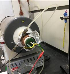
Figure 5: Sample assembly, in the hood fume, with electrodes attached.

7. Open the Zplot software and set the parameters. For this experiment, the parameters will be the same as they were in step 2.
8. Obtain the plots using the same procedure as step 3 (except the z' and z'' values do not need to be compared to the test module). Save the plots.
9. Click the "instant fit" button and choose two points to fit the semi-circle. Use the software to choose the best equivalent circuit model.

Results of EIS are often presented in a Nyquist plot, which shows real impedance versus complex impedance at each frequency tested. The plot of the experiment ran can be seen in Figure 6.

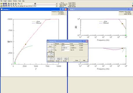
Figure 6: Screenshot of computer after Nyquist plot was obtained. 

As seen in step 9 of the procedure, the software will give you options of circuits to model your data. It is best to choose the simplest model that still accurately reflects the data. Choosing the correct circuit to model the data is a difficult, inverse problem. While software packages exist that can assist in generating model circuits, care should be taken during this analysis.

When an equivalent circuit is chosen, the resulting data can be used to calculate the conductivity of the sample. One way to calculate conductivity is to plot the data from EIS using an Arrhenius model, which plots 1000/T on the x-axis and log(σT) on the y-axis. The data can be fitted to a linear line using the following equation:

    (Equation 5)

Where  for our sample was 374 S/cm*K and E_a, the activation energy, was 0.17 eV, and T = 298 K. Plugging in these values, we calculated a conductivity of 1.67 x 10^-3 S/cm. Previous experiments with this sample reported its conductivity to be approximately 4.1 x 10^-3 S/cm. This is fairly similar to the conductivity value we calculated, indicating that the model we chose was a good, though not perfect, fit.

Electrochemical Impedance Spectroscopy is a useful tool for determining how a new material or device impedes the flow of electricity. It does this by applying an AC signal through the electrodes connected to the sample. The data is collected and plotted by the computer in the complex plain. With the help of software, the graph can be modeled after specific parts of a circuit. This data can often be very complicated and requires careful analysis. This technique, however complex, is an extremely useful non-destructive means of interrogating the real world complexities of electrical impedance, and can provide useful models of how AC current behaves when applied to the sample.

EIS can be used to look at microorganisms in a sample. When bacteria grow on a sample, it can change the electrical conductivity of the sample. Using this idea, you can measure the impedance of a sample at one frequency to determine the population of microorganisms. This technique is known as impedance microbiology.

EIS can also be used to screen for cancer in tissues, known as Tissue Electrical Impedance. The electrical impedance of bodily tissue is determined by its structure. As it degrades over time, it's impedance of electrical current also changes. Much like impedance microbiology, this type of impedance testing looks at the population of cells and can provide useful information about cell heath and morphology.

EIS is also used in the paint and corrosion prevention industries to determine how well a layer is applied to the surface of a material. EIS data corresponds well to every day electrochemical processes that attack surfaces; materials that show an electrical resistance of less than  may not protect against corrosion as well as materials with a higher resistance. EIS is an avenue to predict how new surface treatments will fair in harsh environments without having to recreate them, making it an invaluable tool in the prevention of corrosion which would otherwise cost the United States billions of dollars in repairs every year.