
Mass Conservation and Flow Rate Measurements
Genel Bakış
Source: Ricardo Mejia-Alvarez and Hussam Hikmat Jabbar, Department of Mechanical Engineering, Michigan State University, East Lansing, MI
The purpose of this experiment is to demonstrate the calibration of a flow passage as a flowmeter using a control volume (CV) formulation [1, 2]. The CV analysis focuses on the macroscopic effect of flow on engineering systems, rather than the detailed description that could be achieved with a detailed differential analysis. These two techniques should be considered complementary approaches, as the CV analysis will give the engineer an initial basis on which route to pursue when designing a flow system. Broadly speaking, a CV analysis will give the engineer an idea of the dominant mass exchange in a system, and should ideally be the initial step to take before pursuing any detailed design or analysis via differential formulation.
The main principle behind the CV formulation for mass conservation is to replace the details of a flow system by a simplified volume enclosed in what is known as the control surface (CS). This concept is imaginary and can be defined freely to cleverly simplify the analysis. For instance, the CS should 'cut' inlet and outlet ports in a direction perpendicular to the dominant velocity. Then, the analysis would consist of finding the balance between the net mass flux through the CS and the rate of change of mass inside the CV. This technique will be demonstrated with the calibration of a smooth contraction as a flowmeter.
İlkeler
A control volume (CV) is defined by an imaginary closed surface, dubbed the control surface (CS), defined arbitrarily to study the balance of mass in a system. Figure 1A shows an example of a control volume containing a region of flow going through a flow passage. The details of flow in the passage are irrelevant since we are merely interested in obtaining measures of the mass inflow, outflow, and its rate of change inside the flow passage. All these effects can be summarized in the equation for conservation of mass in integral form [1, 2]:
 (1)
(1)
The first term on the right-hand side of equation (1) represents the rate of change of mass inside the control volume, while the second term represents the net flux of mass through the control surface. The vector difference  is the relative velocity between the CV and the flow, and the vector
  is the unit outward normal to the area differential. The dot product between the relative velocity and represents the velocity component that crosses the CS, and henceforth contributes to the exchange of mass. The sign of this dot product is negative where the mass flux is directed into the CV and positive where it is directed away from the CV.

Figure 1. Schematic of basic configuration. (A) Smooth intake for a centrifugal fan. The control volume is defined as the inside profile of the passage. The solid walls are excluded from the control volume but their boundary conditions are kept in the control surface (i.e. no penetration and no slip). Port 1 is defined as the entrance side of the passage, while port 2 is defined as the cross-sectional plane that coincides with the tip of the Pitot tube. Flow goes from left to right. (B) Pitot-static system and schematic of data acquisition system. Please click here to view a larger version of this figure.
For the present demonstration, we have the configurations shown in Figure 1A, where a fixed CV follows the contour of as smooth contraction at the intake of a centrifugal fan. The flow through this CV is steady, thus the rate of change of mass inside the control volume is zero. Hence, the first term on the right-hand side of equation (1) vanishes. Also, the CV is attached to the contraction, which is fixed in space and has no velocity, making  . Therefore, the net flux of mass through this CV is zero and equation (1) simplifies to:
 (2)
(2)
Considering the configuration in Figure 1A, mass flows into the CV through port 1 and leaves the CV through port 2. Consequently, the surface integral on the right-hand side of equation (2) can be divided into two independent integrals, one for each port. The sign of the dot product is negative in port 1 because the flow goes toward the CV, and positive in port 2 because the flow goes away from the CV. Without assuming that the velocity is homogeneously distributed in either port, let us make  and
and  the respective velocity profiles taking into account that both are what remain after taking the dot product. That is, the magnitude of the velocity component parallel to the area vector, . Finally, pressure changes along the contraction are not significant enough to induce observable changes in density. Henceforth, we can consider the density as constant. Under these circumstances, equation (2) would simplify to:
 (3)
(3)
Note that, since mass is conserved, the mass flux,  , is the same through both ports. Given the structure of these relations, each integral in equation (3) expresses the volumetric flow rate,
 , through its corresponding port, and this fact helps to define the average velocity,
 , for a given port:
 (4)
(4)
Under inviscid conditions, the velocity at port 2 could be expressed in terms of the conditions outside of the intake using Bernoulli's equation along the central streamline (see Figure 1A for reference):
 (5)
(5)
Here, the effect of height vanishes on the central streamline because it is horizontal, and is negligible in the other streamlines because the fluid is air, which has a very small specific weight. Also, the initial point on the central streamline is sufficiently far away from the inlet that its velocity is zero. Given that equation (5) is for the idealized inviscid case, this value of velocity will be the same all across port 2. In reality, boundary layer growth affects the velocity profile and makes it non-homogeneous. To account for this effect, the ideal estimation is compared with experimental measurements via the "Discharge Coefficient". This coefficient is defined as the ratio between the measured average velocity and the inviscid velocity for a given cross section of the flow:
 (6)
(6)
The discharge coefficient,  , depends on the geometry and the Reynolds number. Once determined, could be used in conjunction with equations (4) and (5) to determine the flow rate across port 2 based on its cross-sectional area and an easy-to-measure pressure differential:
 (7)
(7)
When putting equations (4), (5), and (6) together, and considering that port 2 is circular, we obtain the following relationship for :
 (8)
(8)
It is clear from equation (8) that knowledge of the velocity profile is necessary to obtain the discharge coefficient. To this end, we will use velocimetry by Pitot - static probes. As shown in Figure 1B, the Pitot tube brings the flow to a stop sensing the total pressure, , which is the addition of the static and dynamic pressures at a given point. On the other hand, the static probe at the wall senses the static pressure alone. From Bernoulli's equation applied at a given radial position, the total pressure is just Bernoulli's constant. At port 2, this principle can be expressed by the following relation at an arbitrary radial position:
 (9)
(9)
Here, we are neglecting the effect of vertical position because our flow passage is horizontal. In summary, one obtains the following relationship for the magnitude of the velocity at a given position 'r' within the pipe:
 (10)
(10)
The pressure difference  is directly measured by the pressure transducer depicted in Figure 1B, and the velocity profile is obtained by traversing the Pitot tube along the radial coordinate of the pipe. Note that these velocity measurements are carried out at discrete positions, hence, these data points should be used to solve the integral in equation (8) numerically using either the trapezoidal or the Simpson's rule [1]. Once the value of this integral is obtained, it should be plugged into equation (8) together with the measured value of , the density, and the radius of the duct, to obtain the value of for that particular flow condition. Upon repeating this experiment for different flow conditions, we will obtain a scatter plot that could be used to determine a relationship between and . This relationship can then be substituted in equation (7) to fully determine the flow rate,, as a function of solely .
Prosedür
1. Setting the facility
- Make sure that there is no flow in the facility.
- Verify that the data acquisition system follows the schematic in Figure 1B.
- Connect the positive port of pressure transducer #1 (see Figure 1B for reference) to the traversing Pitot tube ().
- Connect the negative port of this same pressure transducer to the static probe of the intake passage (
 ). Hence, the reading of this pressure transducer will be directly (
 ).
). - Record this transducer's conversion factor from Volts to Pascals (
 ). Enter this value in Table 1.
 - Connect the positive port of pressure transducer #2 (see Figure 1B for reference) to the static probe of the intake passage () using a tee.
- Leave the negative port of pressure transducer #2 open to the atmosphere (
 ). Hence, the reading of this transducer will be directly (
 ).
). - Record this transducer's conversion factor from Volts to Pascals (
 ). Enter this value in Table 1.
 - Set the data acquisition system to sample at a rate of 100 Hz for a total of 500 samples (i.e. 5s of data).
- Make sure that channel 1 in the data acquisition system corresponds to pressure transducer #1 ().
- Enter the conversion factor in the data acquisition system to make sure that the pressure measurement () is directly converted to Pascal.
- Set the Pitot probe at the end of its travel, where it touches the pipe's wall. Since the probe is 2 mm in diameter, the first velocity point is at a radial coordinate 1 mm away from the wall. That is, at a radial position of
 mm (here,
 mm).
mm).
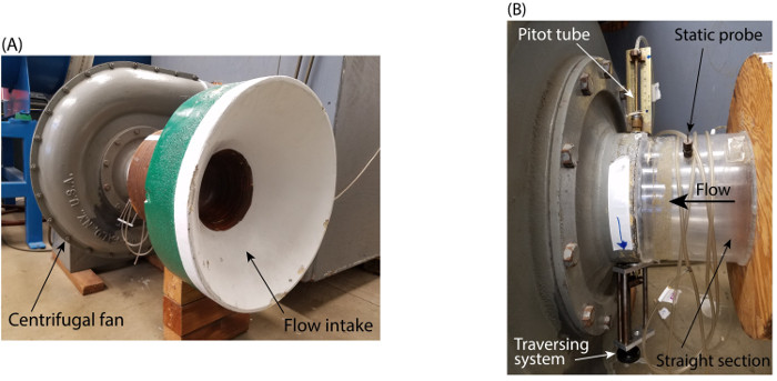
Figure 2. Experimental setting. (A): Flow passage under study. (B): manual traversing system for the Pitot tube. Please click here to view a larger version of this figure.
Table 1. Basic parameters for experimental study. Par ameter Value
| Parameter | Value |
| Flow passage radius (Ro) | 82.25 mm |
| Transducer #1 calibration constant (m_p1) | 136.015944 Pa/V |
| Transducer #2 calibration constant (m_p2) | 141.241584 N/V |
| Local atmospheric pressure | 100,474.15 Pa |
| Local temperature | 297.15 K |
| P_atm-P_2 | 311.01 Pa |
2. Measurements
- Turn the flow facility on.
- Record the reading of pressure transducer #2 in Volts from the digital multimeter.
- Enter this value in Table 1 as and convert the reading from Volts to Pascals using the factor .
- Use the data acquisition system to record the reading of ().
- Enter the value of in Table 2.
- Use the traversing knob to change the radial position of the Pitot tube according to the value suggested in Table 2.
- Repeat steps 2.4 and 2.6 until Table 2 is fully populated.
- Change the flow rate by varying the system's discharge.
- Repeat steps 2.4 to 2.8 for at least ten different flow rates.
- Turn the flow facility off.
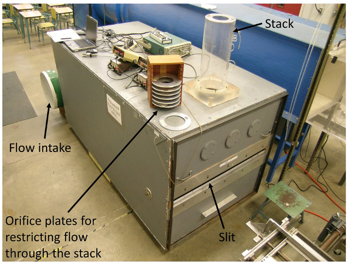
Figure 5. Experimental setting. Perforated plates to restrict flow at the discharge of the flow system. Please click here to view a larger version of this figure.
Table 2. Representative results. Velocity measurements. r (mm) PT - P2 (Pa) u (r) (m/s
| r (mm) | PT - P2 (Pa) | u(r) (m/s) |
| 2.25 | 300.35 | 22.34 |
| 12.25 | 302.84 | 22.43 |
| 22.25 | 305.82 | 22.54 |
| 32.25 | 302.34 | 22.41 |
| 42.25 | 294.88 | 22.13 |
| 52.25 | 295.37 | 22.15 |
| 62.25 | 292.88 | 22.06 |
| 68.25 | 293.63 | 22.09 |
| 72.25 | 294.13 | 22.10 |
| 75.25 | 299.60 | 22.31 |
| 77.25 | 293.13 | 22.07 |
| 79.25 | 284.67 | 21.75 |
| 80.25 | 256.31 | 20.63 |
| 81.25 | 198.33 | 18.15 |
3. Data Analysis.
- Determine the velocity profile using the pressure difference values, PT - P2, from Table 2. Enter the results in Table 2.
- Plot both the pressure and velocity values from Table 2 using the radius,
 , as the abscissas (Figure 3).
 - Calculate the integral in equation (8) based on the velocity and radius values from Table 2.
- Calculate the discharge coefficient for each flow rate using equation (8).
- Plot the discharge coefficient using
 as the abscissas.
 - Fit a function to the discharge coefficient, a power law is a good choice.

Figure 3. Representative results. (A): Example of measurement of static pressure along the radial coordinate of the flow passage. (B): Velocity distribution determined from the measurements of static pressure. Please click here to view a larger version of this figure.
Sonuçlar
For a given restriction of the flow at the fan's discharge, Figure 3A shows the measurements of dynamic pressure () at different radial locations inside the pipe after traversing with the Pitot tube. These values were used to determine the local velocity at those radial locations, and the results are shown in Figure 3B. After using the trapezoidal rule on these data to solve equation (4) for the average velocity, we obtained a value of m/s. On the other hand, the value of from Table 1 was used to determine the ideal velocity from equation (5):
  m/s. Hence, the discharge coefficient for this flow condition is:
  . This value is shown in Figure 4 as a red triangle.
After repeating this experiment twenty-nine more times, we obtained the scatter plot shown in Figure 4. This data can be well represented by a power law of :
 (11)
(11)
The reason for this choice of argument is to make sure that the leading constant stays dimensionless, and hence this correlation would still be valid regardless of the system of units used for the pressure. This function can be substituted in equation (7) to obtain the flow rate as a function of :
:
 (12)
(12)
Here, all the constants of equations (7) and (11) were lumped into a single dimensionless constant: . Consequently, equation (12) is valid for any system of units as long as the variables are consistently assigned the corresponding units. For convenience, the density from equation (7) was expressed in terms of the atmospheric pressure and absolute temperature using the ideal gas law. Equation (12) is valid for different atmospheric conditions as it accounts for changes in local pressure and temperature (T and Patm). Also, as long as geometric similarity is conserved, this equation would be valid for passages of different sizes as accounted by the radius R.
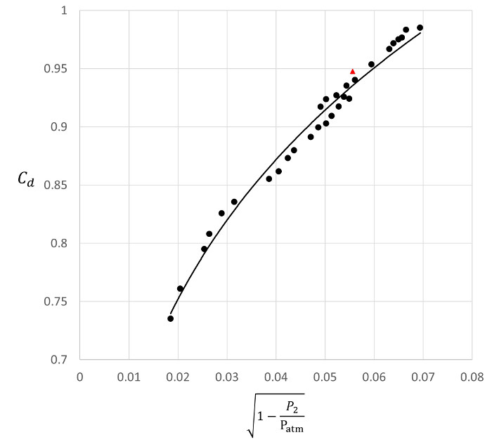
Figure 4. Representative results. : Discharge coefficients determined at different flow rates.
  : Discharge coefficient determined with the velocity measurements demonstrated herein. - : Power law fitted to the experimental data.
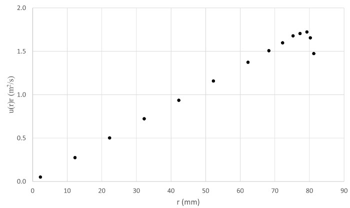
Figure 6. Representative results. Plot of the product between velocity and radius.
Table 3. Representative results. Discharge coefficient.
| √(1-P2/Patm ) | Cd |
| 0.019 | 0.735 |
| 0.020 | 0.761 |
| 0.025 | 0.795 |
| 0.026 | 0.808 |
| 0.029 | 0.826 |
| 0.032 | 0.835 |
| 0.039 | 0.855 |
| 0.041 | 0.862 |
| 0.042 | 0.873 |
| 0.044 | 0.880 |
| 0.047 | 0.891 |
| 0.049 | 0.899 |
| 0.049 | 0.917 |
| 0.050 | 0.924 |
| 0.050 | 0.903 |
| 0.051 | 0.909 |
| 0.052 | 0.927 |
| 0.053 | 0.917 |
| 0.054 | 0.926 |
| 0.054 | 0.935 |
| 0.055 | 0.924 |
| 0.056 | 0.940 |
| 0.060 | 0.953 |
| 0.063 | 0.967 |
| 0.064 | 0.972 |
| 0.065 | 0.975 |
| 0.066 | 0.977 |
| 0.067 | 0.983 |
| 0.069 | 0.985 |
Başvuru ve Özet
We demonstrated the application of control volume analysis of conservation of mass to calibrate a flow passage as a flow meter. To this end, we demonstrated the use of a Pitot-static system to determine the flow rate across the flow passage using integration over the velocity profile. Then, the concept of discharge coefficient was incorporated to account for the effect of boundary layer growth near the walls of the flow passage. Based on a set of velocity measurements for different flow rates, we developed a regression that expresses the discharge coefficient as a function of the ratio between the static pressure at the flow passage and the local atmospheric pressure,. Finally, this regression was incorporated into an equation for the flow rate through the passage as a function of. This equation was developed to keeps its validity under changes in local atmospheric conditions, passage size, and unit system.
Control volume analysis for mass conservation offers many alternatives to calibrate flow passages as flowmeters. For example, perforated plates, nozzles, and venturi tubes are used in confined flows to determine flow rate based on pressure changes between two different sections of the passage. And similar to our example, these devices need to be characterized with a discharge coefficient that corrects for boundary layer effects.
In flow through open channels, control volume analysis for mass conservation can also be used to assess flow rate by comparing the depth of flow before and after flow restrictions such as spillways, partially open gates, or cross-section reductions. The main significance of these applications is that hydraulic structures for water distribution, control, and treatment are of very large scales that would preclude the use of other flow devices.
Atla...
Bu koleksiyondaki videolar:

Now Playing
Mass Conservation and Flow Rate Measurements
Mechanical Engineering
22.9K Görüntüleme Sayısı

Buoyancy and Drag on Immersed Bodies
Mechanical Engineering
30.2K Görüntüleme Sayısı

Stability of Floating Vessels
Mechanical Engineering
23.2K Görüntüleme Sayısı

Propulsion and Thrust
Mechanical Engineering
22.1K Görüntüleme Sayısı

Piping Networks and Pressure Losses
Mechanical Engineering
58.8K Görüntüleme Sayısı

Quenching and Boiling
Mechanical Engineering
8.2K Görüntüleme Sayısı

Hydraulic Jumps
Mechanical Engineering
41.3K Görüntüleme Sayısı

Heat Exchanger Analysis
Mechanical Engineering
28.3K Görüntüleme Sayısı

Introduction to Refrigeration
Mechanical Engineering
25.0K Görüntüleme Sayısı

Hot Wire Anemometry
Mechanical Engineering
15.9K Görüntüleme Sayısı

Measuring Turbulent Flows
Mechanical Engineering
13.6K Görüntüleme Sayısı

Visualization of Flow Past a Bluff Body
Mechanical Engineering
12.2K Görüntüleme Sayısı

Jet Impinging on an Inclined Plate
Mechanical Engineering
10.8K Görüntüleme Sayısı

Conservation of Energy Approach to System Analysis
Mechanical Engineering
7.4K Görüntüleme Sayısı

Determination of Impingement Forces on a Flat Plate with the Control Volume Method
Mechanical Engineering
26.0K Görüntüleme Sayısı
JoVE Hakkında
Telif Hakkı © 2020 MyJove Corporation. Tüm hakları saklıdır