Just-noticeable Differences

Source: Laboratory of Jonathan Flombaum—Johns Hopkins University

Psychophysics is a branch of psychology and neuroscience that tries to explain how physical quantities are translated into neural firing and mental representations of magnitude. One set of questions in this area pertains to just-noticeable differences (JND): How much does something need to change in order for the change to be perceivable? To pump intuitions about this, consider the fact that small children grow at an enormous rate, relatively speaking, but one rarely notices growth taking place on a daily basis. However, when the child returns from sleep-away camp or when a grandparent sees the child after a prolonged absence, just a few weeks of growing is more than perceptible. It can seem enormous! Changes in height are only noticed after an absence because the small changes that take place on a day-to-day basis are too small to be perceivable. But after an absence, many small changes add up. So how much growth needs to take place to be noticeable? The minimal amount is the JND.

Psychologists and neuroscientists measure JND in many domains. How much brighter does a light need to be to be noticed? How much louder does a sound need to be? They often obtain the measurements by employing a forced-choice paradigm. This video will focus on size, demonstrating a standard approach for measuring a JND when the area of a shape changes.

1. Equipment

1. For this experiment, use a computer and experiment implementation software such as E-Prime, or a programming environment such as MATLAB or PsychoPy.

2. Stimuli and Experiment Design

1. This experiment will involve repeated trials with the same basic design. Two discs will appear on the screen simultaneously, one on the left side and one on the right. One will always be bigger than other, and the task will be to use a keypress to select the larger one. The details are as follows:
2. Program the experiment to draw a blue disc with a radius of 10 px. The disc will appear in each trial of the experiment, centered in the display vertically, and centered horizontally in either the left or right half of the display. Using one stimulus that appears unchanged in every trial is sometimes called the method of constant stimulus. It just refers to the fact that one of the two stimuli in each trial is always the same. The 10-px blue disc is thus the constant stimulus.
3. Opposite the constant stimulus in each trial, display another blue disc. This disc is called the comparison stimulus. It will have a radius between 5 and 9 and between 11 and 15 px. That is 10 total possibilities. In the experiment, include 10 trials each for each of the 20 possible comparison stimuli. So the experiment will involve 200 trials.
4. Display the two stimuli on the screen for 200 ms, followed by a screen which reads only 'Which was bigger L/R?' Figure 1 schematizes the sequence of events in each trial.
   1. 'L' key responses will indicate that the left object was bigger, and 'R' key responses will designate that the right one was perceived as bigger.
5. Be sure that the program outputs the following important data into a table: the trial number, the size of the comparison stimulus, the screen position of the comparison stimulus, the correct response, and the response given by the participant. Figure 2 shows a sample of such a data table.

Figure 1. A schematic depiction of a single forced-choice trial in an experiment to measure the Just-noticeable difference (JND) for circle size. First, a ready screen prompts the participants that a trial will begin. Next, two blue discs appear in the display, side-by-side. They remain present for only 200 ms, at which point the display prompts the participant for a response. The 'L' key is used to indicate the object on the left, and the 'R' key to indicate the object on the right.

Figure 2. A sample output table from a forced-choice JND experiment. The columns report the relevant data from the experimental program.

3. Running the experiment

1. Recruit a participant, and when she arrives in the lab tell her that she will do a simple experiment on the perception of shape. Then have her complete informed consent.
2. Seat the participant in front of the testing computer, and explain the task as follows:
   1. Every trial of this experiment will involve the same basic sequence of events. First, you will see the word 'Ready?' on the screen. Press spacebar when you are ready to begin the trial. At that point, two blue discs will appear on either side of the screen very briefly. When they disappear, the display will read 'Which was bigger, L/R?' Your job is to report which of the two discs looked bigger to you, the one on the right or the one on the left side of the screen. There are 200 trials in the experiment, but they are short. The whole experiment should take under five minutes. Do you have any questions?
3. After answering any questions, launch the experimental program, and let the participant begin. Leave her in the quiet testing room until the experiment is complete.

4. Analyzing the results

1. To analyze the results, the first thing to do is determine which responses were correct and which were incorrect. Add a column to the data output table for these purposes. Compare the response given and the correct response, marking the final column with a 1 when the response given was correct and 0 when it was not.
   1. Quickly look to make sure that performance was sensible-that the participant was at or near perfect accuracy when the comparison was 5 and 15 px, differences large enough compared to 10 that no errors should have been made.
2. Now add another column to the data table, called 'Proportion of C Responses.' In the column, note whether the comparison or the constant was chosen by the participant. If the comparison object was chosen, mark a 1 in the column. If the constant was chosen, mark a 0.
3. Now, for each comparison size, compute the fraction of the time that the comparison was selected as larger by the participant. For comparison stimuli of 5, the number should be close to 0, and for comparison stimuli of 15 it should be close to 1.
4. To visualize the results, graph them as follows: Make scatter plot, with the size of the comparison on the x-axis and the proportion of times it was chosen on the y-axis. It will look something like the one in Figure 3.

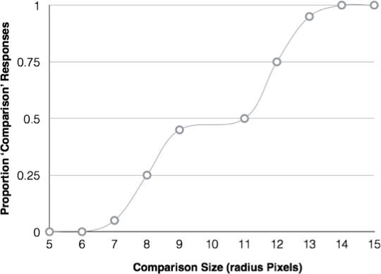
Figure 3. Results of a forced-choice experiment to find the JND for circle radius. Plotted is the proportion of time that the comparison stimulus was selected as larger (by the participant) as a function of the size of the comparison stimulus. The constant stimulus always had a radius of 10 px.

The graph in Figure 3 shows the proportion of time in which the comparison stimulus was chosen as a function of the size of its radius. Recall that the constant stimulus always has a 10-px radius in this experiment. This is why with a radius of 5 or 6 px the comparison is almost never chosen, and it is almost always chosen with a radius if 14 or 15 px. However, with a radius of 9 or 11 px, the comparison is difficult. Participants often make mistakes. The JND is defined as follows: The comparison size when it is chosen about 75% of the time minus its size when it is chosen 25% of the time, all divided by 2. Here, those numbers are 12 and 8, respectively. So the JND for circle radius is 2 px.

There are detailed mathematical reasons for why this is the exact calculation of a JND, having to do with statistics and the nature of normal distributions (bell curves). But looking at the graph should make the computation more intuitive. When the radius was only 1 px smaller or bigger than 10, the participant made many mistakes, performing very near 0.5, which is what she would produce if she were just guessing. But performance quickly became far more accurate with a pixel difference of 2, and it was nearly perfect with a pixel difference of 3 or larger. Figure 4 is an annotated version of Figure 3, meant to illustrate the calculation of a JND.

Figure 4. An annotated version of Figure 3.

One of the main applications of the constant stimulus approach to measuring a JND has come in neuroscience, specifically in neurophysiology studies devised to investigate how the firing of individual neurons encodes physical properties about the world. These studies usually involve a monkey with electrodes implanted in their visual cortex. The electrodes penetrate individual cells that respond to visual stimulation by firing or spiking, that is, by conducting a rapid electrical signal. In studies on using JND methods, researchers have discovered that individual neurons are noisy-they respond to the size or brightness or color of a stimulus more or less the same way every time, but with some variability. The result is that two very similar stimuli will elicit the same response some of the time. A circle with a radius of 10 px will sometimes get the same neuronal response as a circle with a radius of 9 px or a circle with a radius of 11 px. This is why JND are just-barely-noticeable: sometimes, in the brain, the relevant stimuli really do produce indistinguishable effects.