
Determination of Impingement Forces on a Flat Plate with the Control Volume Method
Overview
Source: Ricardo Mejia-Alvarez and Hussam Hikmat Jabbar, Department of Mechanical Engineering, Michigan State University, East Lansing, MI
The purpose of this experiment is to demonstrate forces on bodies as the result of changes in the linear momentum of the flow around them using a control volume formulation [1, 2]. The control volume analysis focuses on the macroscopic effect of flow on engineering systems, rather than the detailed description that could be achieved with a differential analysis. Each one of these two techniques have a place in the toolbox of an engineering analyst, and they should be considered complementary rather than competing approaches. Broadly speaking, control volume analysis will give the engineer an idea of the dominant loads in a system. This will give her/him an initial feeling about what route to pursue when designing devices or structures, and should ideally be the initial step to take before pursuing any detailed design or analysis via differential formulation.
The main principle behind the control volume formulation is to replace the details of a system exposed to a fluid flow by a simplified free body diagram defined by an imaginary closed surface dubbed the control volume. This diagram should contain all surface and body forces, the net flux of linear momentum through the boundaries of the control volume, and the rate of change of linear momentum inside the control volume. This approach implies cleverly defining the control volume in ways that simplify the analysis at the same time that capture the dominant effects on the system. This technique will be demonstrated with a plane jet impinging on a flat plate at different angles. We will use control volume analysis to estimate the aerodynamic load on the plate, and will compare our results with actual measurements of the resulting force obtained with an aerodynamic balance.
Principles
A control volume (CV) is defined by an imaginary closed surface, dubbed the control surface (CS), defined arbitrarily to study the effect of flow around objects and systems. Figure 1 shows an example of a control volume containing a region of flow going around a solid object. The flow in the immediate vicinity of the object is highly complex, and we would like to avoid that complexity in order to estimate the global effect of the flow on the supporting element. Once defined, the CV becomes a free body diagram that captures the interactions between the flow and the enclosed object that give rise to loads in the supporting system. To this end, we equate the surface and body forces on the CV with the change of linear momentum of the flow that goes through the CV. The surface forces are pressure, flow-induced shear, and any reactions of the solids "cut" by the control volume. The body forces are basically the weight of everything contained in the control volume, including solids and fluids, and any other force induced by volumetric effects such as electromagnetic fields. The change in linear momentum of the flow is the added effect of the net flux of momentum through the CS and the rate of change of momentum contained in the CV. All these effects can be summarized in the equation for conservation of linear momentum in integral form:
 (1)
(1)
Here,  are the surface forces and
  are the body forces. The first term on the right-hand side of equation (1) represents the rate of change of momentum inside the control volume, while the second term represents the net flux of momentum through the control surface. The vector difference
  is the relative velocity between the CV and the flow, and the vector
  is the unit outward normal to the area differential. The dot product between the relative velocity and represents the velocity component that crosses the CS, and henceforth contributes to the exchange of linear momentum. The sign of this dot product is negative where the momentum flux is directed into the CV and positive where it is directed away from the CV. In this form, equation (1) is the balance of linear momentum in relation to an inertial frame of reference. Note that (1) is a vector equation, which means that in general is has three independent components. With this in mind, the analyst needs to be careful at establishing the set of forces that balance changes in linear momentum for each coordinate.
For the present demonstration, we have the configuration shown in Figure 1, where a fixed CV encloses a plate that is exposed to a plane jet. Since the jet flow is steady, there is no change of momentum inside the CV, so the first term on the right-hand side of equation (1) vanishes. Also, the CV does not move, so  . Hence, the summation of forces on the CV balances with the net flux of momentum through the CS.
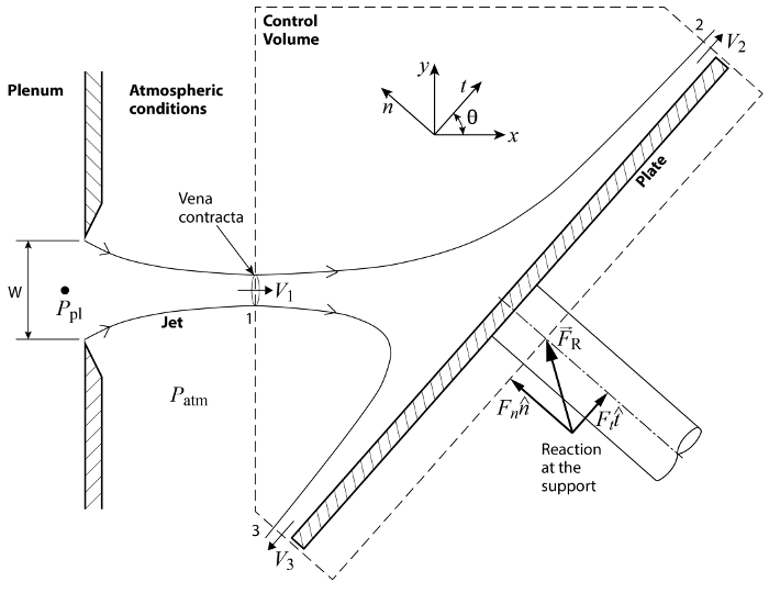
Figure 1. Schematic of basic configuration. A plane jet exits the plenum through a slit of width W. The jet impinges on an inclined plate and it gets deflected while exerting a load on the surface.
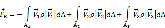
Considering the configuration in Figure 1, momentum flows into the CV through port 1 and leaves the CV through ports 2 and 3. The CV crosses the incoming jet at the vena contracta, (for more information, please see video "The Interplay of Pressure and Velocity: jet impinging on an inclined plate") which is the first place at which the streamlines become parallel and, as a result, the static pressure across the jet becomes homogeneous and matches the value of the surrounding pressure, that is, atmospheric pressure  . Similarly, ports 2 and 3 are located far enough from the impinging region to allow for the streamlines to become parallel and the pressure to match that of the surroundings. As a result, the pressure everywhere on the CS is equal to the atmospheric pressure, . In consequence, given that the pressure is homogeneously distributed around the CS, its net force on the control volume is zero. Additionally, since the CS was drawn perpendicular to the inlet and outlet flows, there is not any shear load induced by the flow on the CS. In summary, equation (1) simplifies to the following relationship for the case illustrated in Figure 1
 (2)
(2)
Here,  is the reaction of the supporting system resulting from transmission of the aerodynamic loading that the jet exerts on the plate. As shown in Figure 1, this reaction is located at the portion of the control volume that "cuts" through the supporting system of the plate. This is considered a surface force in the sense that this imaginary cut would be part of the control surface. Since is the only interaction with the control volume not associated with momentum flux, it is the only term on the left-hand side of equations (1) and (2). Note from comparing these equations with each other that the dot products inside the integrals result simply in the magnitudes of the corresponding velocity vectors because they are aligned with the area vectors. Also, as said before, their sign tells if the momentum flux is directed into the CV (-) or away from it (+). If we further assume that the velocity at the ports is approximately homogeneous, and that the flow is incompressible, the velocities and density can be taken outside of the integrals and equation (2) becomes:
 (3)
(3)
Rigorously speaking, the velocity profile is never perfectly homogeneous, and this simplification requires a multiplication by a correction coefficient,  , whose value depends on the details of the velocity profile. At a given flux port, this coefficient is defined as the ratio between the exact momentum flux and the momentum flux estimated from the average velocity:
 (4)
(4)
In turbulent flows this coefficient is very close to 1 because the velocity profile tends to be close to homogeneous. Since this is the case for the present experiment, equation (3) is a reasonable approximation for the current measurements. But if the flow rate were to be reduced or the position of the plate moved farther downstream until reaching laminar flow conditions, it would be necessary to solve the integrals on the right-hand side of equation (2) without approximation. Based on Figure 1, can be decomposed in its normal and tangent coordinates to the plate  . Where
  and
and  are the unit vectors in each coordinate and
  and
and  are the magnitudes of the projections of in each coordinate. Hence, equation (3) can be decomposed as:
 (5)
(5)
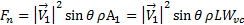
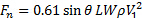
Note that the minus sign on the normal component disappears because the projection of on the normal axis is negative. We want to determine the normal load on the plate with this study because it tends to be the most relevant component from the structural point of view. From equation (4), we obtain the normal load on the plate:
 (6)
(6)
Here,  is the plate span and
  is the width of the jet at the vena contracta. In general, the contraction ratio between the jet exit width,
  , and the vena contracta is very close to [2, 3, 4]:
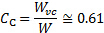 (7)
(7)
In summary, the normal force on the plate can be estimated from the following relationship:
 (8)
(8)
Here, we define  for simplicity. On the other hand, the value of the term
  is determined using Bernoulli's equation between the plenum and the vena contracta (see Figure 2 for reference). The velocity inside the plenum is considered negligible, and given that the jet is horizontal, changes in height between the plenum and the vena contracta vanish. Hence, Bernoulli's equation becomes:
 (9)
(9)
Recall that the pressure at the vena contracta matches the surrounding pressure, which is atmospheric. Hence, the dynamic pressure at the vena contracta follows:
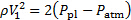 (10)
(10)
Substituting equation (9) in equation (7) gives the final result to estimate the normal force on the plate based on the characteristics of the plane jet:
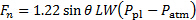 (11)
(11)
This result comes from the control volume analysis of conservation of linear momentum. To have an assessment of its accuracy, we will compare these estimations to direct measurements of the force. To this end, the horizontal ( and vertical (
 components of the total force depicted in Figure 2 are captured by an aerodynamic balance. To determine the components of this measured force on the
  coordinate system, we use the following coordinate transformation:
 (12)
(12)
 (13)
(13)
Where a tilde was added to emphasize that these forces are obtained by direct measurement with an aerodynamic balance.
Procedure
1. Setting the facility
- Make sure that there is no flow in the facility.
- Connect the positive port of the pressure transducer to the plenum pressure tap (
 ).
). - Leave the negative port of the pressure transducer open to the atmosphere ().
- Record the transducer's conversion factor from Volts to Pascals (
 ).
). - Record the jet exit width.
- Record the plate span.
- Record the force balance's conversion constants from Volts to Newton (horizontal force:
 ; vertical force:
  ).
). - Setup the data acquisition system to sample at a rate of 100 Hz for a total of 1000 samples (i.e. 10s of data).
- Mount the impact plate on the force balance and adjust its outputs to zero.
2. Recording the data
- Set the angle of the plate to 90o (see Figure 2 for reference).
- Turn the flow facility on.
- Record the reading of the pressure transducer in Volts, which corresponds to the pressure difference between the Plenum and the atmosphere (
 ).
). - Record the force data using the data acquisition system.
- Multiply the acquired values (in Volts) by the force conversion factors ( and ) and enter the results in table 1.
- Turn the flow facility off.
- Change the angle of the plate.
- Repeat steps 2.2 to 2.6 for the following angles:


Figure 2 . Experimental setting. (A): Detail of intake system to pressurize the plenum at pressure  . (B): discharge side with impingement plate. (C): Detail of discharge slit. Please click here to view a larger version of this figure.
3. Data Analysis
- Calculate the normal force measured by the balance using equation(11) and record it in table 1.
- Determine the theoretical value of the normal force from equation (10) and record it in table 1.
- Calculate the disagreement between the two values as a percent.
Table 1 . Basic parameters for experimental study.
| Parameter | Value |
| Jet nozzle width (W) | 19.05 mm |
| Plate span (L) | 110.49 cm |
| Transducer calibration constant (m_p) | 141.3829 Pa/V |
| Balance horizontal coefficient (m_x) | 22.2411 N/V |
| Balance vertical coefficient (m_y) | 4.4482 N/V |
Results
Figure 3 shows a comparison between the normal load on the flat plate as measured directly from an aerodynamic balance and estimated from conservation of linear momentum. In general, the analysis of linear momentum captured the dominant tendency of direct measurements as the impingement angle changes. The discrepancies in these measurements varied non-monotonically with the impingement angle. For impingement angles in the range  , and for
  , discrepancies are below 6%. They are higher for the other angles, but never higher than 12.5%. There appears to be a crossover around
  , in which the tendency of discrepancies invert: measurements exhibit higher normal loads than analysis of linear momentum for
  and lower for
  . These differences in the tendencies could be due to the fact that the analysis of linear momentum assumes inviscid, non-dissipative, changes in linear momentum, while direct measurements cannot avoid the effect of viscosity on the flow. For the range , the shear component becomes dominant and therefore turbulent boundary layer effects could be important. In this case, wall-normal velocity fluctuations due to turbulence might be responsible for the increase in the normal load. On the other hand, the axial velocity of the jet experiences a significant reduction in the range while it turns to become dominantly tangent to the wall. This effect is likely to let viscosity dissipate viscosity due to a reduction in the local values of Reynolds number, and that would result in reduced values of the normal load.
Table 2. Representative results.
| θ | F ̃_x(N) | F ̃_y (N) | F ̃_n (N) | F_n (N) | ε (%) |
| 90o | 15.257 | 9.034 | 15.257 | 16.773 | 9.9 |
| 85o | 15.151 | 9.831 | 15.950 | 16.709 | 4.8 |
| 82.5o | 15.035 | 10.231 | 16.242 | 16.630 | 2.4 |
| 80o | 15.929 | 10.498 | 17.510 | 16.518 | 5.7 |
| 75o | 14.248 | 10.453 | 16.468 | 16.202 | 1.6 |
| 70o | 13.518 | 11.405 | 16.604 | 15.762 | 5.1 |
| 67.5o | 13.100 | 11.294 | 16.425 | 15.496 | 5.7 |
| 65o | 12.771 | 11.579 | 16.468 | 15.202 | 7.7 |
| 60o | 11.881 | 11.863 | 16.221 | 14.526 | 10.5 |
| 50o | 9.746 | 11.241 | 14.691 | 12.849 | 12.5 |
| 40o | 6.357 | 9.444 | 11.320 | 10.782 | 4.8 |
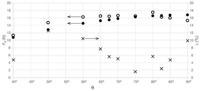
Figure 3. Representative results. Load on plate as a result of impinging jet. Symbols represent:  : direct load measurement;
  : estimation from conservation of linear momentum;
  : percent error between experimental measurements and theoretical estimation.
Application and Summary
We demonstrated the application of control volume analysis of conservation of linear momentum to determine the forces exerted by a jet impinging on a flat plate. This analysis proved simple to apply, and gave a satisfactory bulk estimation of loads without requiring detailed knowledge of the flow pattern around the plate. Though there were some discrepancies (both in magnitude as well as tendency) due to the basic assumption of inviscid transformation of momentum, this technique offers a means of obtaining a quick estimation of system behavior without delving into a detailed study of fluid flow. Hence, this is a powerful tool for the engineering analyst to, for instance, predict the feasibility of developing a given engineering system with a minimal investment of time and resources. Once this first analysis is conducted to determine feasibility, the engineer can move into a more detailed flow analysis using, for example, computational fluid dynamics.
Control volume analysis of conservation of linear momentum is a powerful tool for fluids engineering. It finds application in a wide variety of problems to circumvent more involved methods such as differential analysis. A few instances of this analysis can be described:
Pelton turbine blade design: in general, a Pelton turbine blade should be designed to convert the highest amount of linear momentum into torque. This is achieved by determining the geometry of the blade that maximizes the change in the linear momentum of water jets. To this end, the typical result of control volume analysis is that the jet should be made to turn around on itself, that is, 180o. This is in general a technical challenge for a rotating device, but gives the analyst an initial guidance for a more detailed analysis using other tools.
Drag load on civil structures: one of the challenges of civil engineering is to design structures that stand the load of wind. In order to predict the effects of the wind on a real-size structure, it is possible to conduct experiments with a down-scaled model in wind or water tunnels. To this end, it is possible to use control volume analysis of conservation of linear momentum based on velocity measurements upstream and downstream of the model to determine the effective load on the prototype. This method both simplifies the experimental campaign and saves time, effort, and money in preparation for the construction of a real-scale structure.
Skip to...
Videos from this collection:

Now Playing
Determination of Impingement Forces on a Flat Plate with the Control Volume Method
Mechanical Engineering
26.0K Views

Buoyancy and Drag on Immersed Bodies
Mechanical Engineering
30.2K Views

Stability of Floating Vessels
Mechanical Engineering
23.1K Views

Propulsion and Thrust
Mechanical Engineering
22.1K Views

Piping Networks and Pressure Losses
Mechanical Engineering
58.7K Views

Quenching and Boiling
Mechanical Engineering
8.2K Views

Hydraulic Jumps
Mechanical Engineering
41.3K Views

Heat Exchanger Analysis
Mechanical Engineering
28.3K Views

Introduction to Refrigeration
Mechanical Engineering
25.0K Views

Hot Wire Anemometry
Mechanical Engineering
15.8K Views

Measuring Turbulent Flows
Mechanical Engineering
13.6K Views

Visualization of Flow Past a Bluff Body
Mechanical Engineering
12.1K Views

Jet Impinging on an Inclined Plate
Mechanical Engineering
10.8K Views

Conservation of Energy Approach to System Analysis
Mechanical Engineering
7.4K Views

Mass Conservation and Flow Rate Measurements
Mechanical Engineering
22.9K Views
Copyright © 2025 MyJoVE Corporation. All rights reserved