Constant Temperature Anemometry: A Tool to Study Turbulent Boundary Layer Flow

Source: Xiaofeng Liu, Jose Roberto Moreto, and Jaime Dorado, Department of Aerospace Engineering, San Diego State University, San Diego, California

A boundary layer is a thin flow region immediately adjacent to the surface of a solid body immersed in flow field. In this region, viscous effects, such as the viscous shear stress, dominate, and the flow is retarded due to the influence of friction between the fluid and the solid surface. Outside of the boundary layer, the flow is inviscid, i.e., there is no dissipative effects due to friction, thermal conduction or mass diffusion.

The boundary layer concept was introduced by Ludwig Prandtl in 1904, which enables significant simplification to the Navier-Stokes (NS) equation for the treatment of flow over a solid body. Inside the boundary layer, the NS equation is reduced to the boundary layer equation, while outside of the boundary layer, the flow can be described by the Euler equation, which is a simplified version of the NS equation.

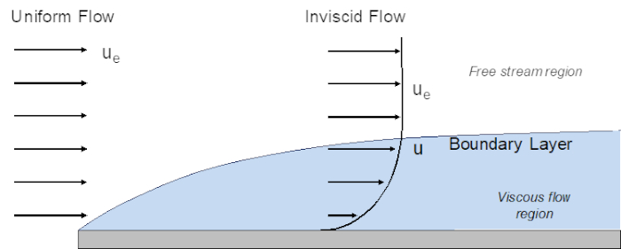
Figure 1. Boundary layer development over a flat plate.

The simplest case for boundary layer development occurs on a flat plate at zero angle of incidence. When considering boundary layer development on a flat plate, the velocity outside of the boundary layer is constant so that the pressure gradient along the wall is considered to be zero.

The boundary layer, which naturally develops on a solid body surface, typically undergoes the following stages: first, the laminar boundary layer state; second, the transition state, and third, the turbulent boundary layer state. Each state has its own law(s) describing the flow structure of the boundary layer.

The research into the development and structure of boundary layer is of great importance for both theoretical study and practical applications. For example, boundary layer theory is the basis for calculating the skin friction drag on ships, aircraft and the blades of turbomachines. Skin friction drag is created on the body surface within the boundary layer and is due to the viscous shear stress exerted on the surface through fluid particles in direct contact with it. The skin friction is proportional to the fluid viscosity and the local velocity gradient on the surface in the surface normal direction. Skin friction drag is present on the entire surface, thus it becomes significant over large areas, such as an airplane wing. Additionally, turbulent fluid flow creates more skin friction drag. The macro-turbulent fluid motion enhances the momentum transfer within the boundary layer by bringing fluid particles with high momentum down to the surface.

This demonstration focuses on the turbulent boundary layer over a flat plate, in which the flow is irregular, such as in mixing or eddying, and the fluctuations are superimposed on the mean flow. Thus, the velocity at any point in a turbulent boundary layer is a function of time. In this demonstration, constant temperature hot-wire anemometry, or CTA, will be used to conduct a boundary layer survey. Then, the Clauser chart method will be used to calculate the skin friction coefficient in a turbulent boundary layer.

A turbulent flow is one in which irregular fluctuations, such as mixing or eddying motions, are superimposed on the mean flow. The velocity at any point in a turbulent boundary layer is a function of time. The fluctuations can occur in any direction of the flow field, and they affect macroscopic lumps of fluid. Thus, whereas momentum transport occurs on a microscopic (or molecular) scale in a laminar boundary layer, it occurs on a macroscopic scale in a turbulent boundary layer. The size of these macroscopic lumps determines the scale of the turbulence.

The effects caused by the fluctuations are as if the viscosity were increased. As a result, the shear forces at the wall and the skin-friction component of the drag are much larger when the boundary layer is turbulent. However, since a turbulent boundary layer can negotiate an adverse pressure gradient for a longer distance, boundary layer separation may be delayed or even avoided altogether.

When describing a turbulent flow, it is convenient to express the local velocity components as the sum of a mean motion plus a fluctuating motion:

where is the time-averaged value of the u component of velocity, and is the velocity of the fluctuation. The time-averaged value at a given point in space is calculated as:

The integration interval, Δt, should be much larger than any significant period of the fluctuation velocity, , so as to converge to a mean velocity value. Thus, by definition, the converged mean value is independent of time, i.e., .

For a boundary layer on a flat plate, the external velocity is a constant. Therefore the pressure gradient term is zero. Even with this simplification, there is no exact solution for a turbulent boundary layer. However, through extensive experimental and analytical investigations on the boundary layer, the flow structure and the empirically-determined relationships describing the profile of the tangential component of the mean velocity have been established.

Very near the wall, the viscous shear dominates. To a first order, the velocity profile is linear; that is, is proportional to y. Thus, the wall shear stress can be expressed as:

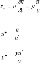
where is called the skin-friction velocity and is defined as:

where τ_w is the skin friction, i.e., the wall shear stress. The skin friction is usually expressed in terms of the skin friction coefficient, C_f, which is defined as:

With these definitions, it is clear that for the laminar sublayer, the following relation is valid:

In the laminar sublayer, the velocity is so small that viscous forces dominate and there is no turbulence. The edge of the laminar sublayer corresponds to a y⁺ of 5 to 10.

In 1933, Prandtl deduced that the mean velocity in the inner region of the boundary layer must depend on the wall shear stress, i.e., skin friction, the fluid physical properties, and the distance, y, from the wall. The velocity in the inner region is thus described by the log law-of-the-wall:

In 1930, Von Kármán deduced that in the outer region of the turbulent boundary layer, the mean velocity, , is reduced below the free-stream value, , in a manner that is independent of the viscosity but is dependent on the wall shear stress and the distance, y, over which its effect has diffused. The velocity in the outer region is given by:

which is known as Law of the Wake. In this equation, is the boundary layer thickness, and is the skin-friction velocity, which is defined as:

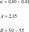
For incompressible flow past a flat plate, the constants are defined as follows:

A suitable technique to measure turbulent boundary layer properties is by hot-wire anemometry, which is based on two principles related to the cooling effect of flow on a heated wire. The first principle is based on the heat transfer of a flow over a surface. When a fluid flows over a hot surface, the convective heat coefficient changes, which in turn affects the heat exchange rate on that surface, and consequently, may further affect the surface temperature.

The second principle is Joule's law, which states that the heat dissipation from an electrical conductor is proportional to the electric potential that is applied to the electrical conductor, squared as shown in the following equation:

where is the heat flux, I is the electric current through a conductor, R is the electrical resistance of the conductor, and U is the electric potential. One may use these two principles to correlate the velocity of fluid flow surrounding a heated metallic wire probe by measuring the electric potential applied to the probe terminals. The applied potential can be used to maintain a constant current through the wire, which is constant current anemometry or CCA, or a constant temperature on the wire, which is constant temperature anemometry or CTA.

In this demonstration, we use constant temperature anemometry (CTA) to conduct a turbulent boundary layer survey. CTA is a widely-used conventional flow diagnostic technique that has a high frequency response and can measure the small scales of turbulence without large interferences. The CTA technique utilizes a very thin metallic wire (≈ 5 μm, usually made of platinum or tungsten), which is connected to an arm of a Wheatstone bridge (Figure 2). The wire is heated to a constant temperature by applying an electrical current. Any cooling is caused by fluid flow around the wire. The Wheatstone bridge controls the electric potential applied to the wire in response to the flow velocity changes so that the heated wire resistance, and therefore the wire temperature, is held constant. The electric potential change of the Wheatstone bridge defines the signal output of the CTA.

Thus, the change in the bridge potential is a function of the heat transfer coefficient, where the heat transfer coefficient is a function of the velocity. We can obtain an empirical correlation between the airspeed and the electric potential of the bridge by calibrating the hot-wire apparatus experimentally. This involves fitting the experimental data using known heat transfer relationships.

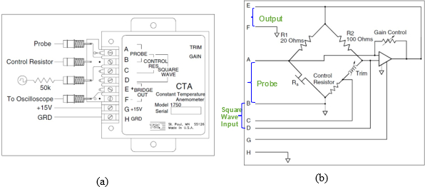
Figure 2. TSI constant temperature anemometer model 1750. (a) Anemometer and cable connectors. (b) Electric circuit diagram, in which Rs represents the hot-wire probe.

Once air speed is calculated using CTA, we can deduce the skin friction coefficient, C_f, on the flat plate. Unfortunately, direct measurement of the skin friction drag is not available, therefore, indirect methods are used to determine its value. The Clauser Chart method is one such method. In the Clauser chart method, the measured value of the skin-friction coefficient, C_f, is determined by comparing the measured boundary layer velocity profile with a family of curves derived from the log law-of-the-wall with prescribed skin-friction coefficient values. The curve that best overlaps with the log law portion of the measured velocity profile on the semi-log plots gives the value of the measured skin friction coefficient.

1. Hot-wire system dynamic response determination

The purpose of this procedure is to understand how fast the anemometer system can respond to flow signal changes. This capability is gauged by measuring the frequency response when the signal turns on and off by applying a square wave.

1. Secure the hot wire probe of the CTA system inside of a wind tunnel using a support shaft.
2. Set-up a DC power supply, signal generator and oscilloscope and connect them as shown in Figure 2(a). The signal generator supplies a square wave input to the Wheatstone bridge, and the output waveform is visualized on the oscilloscope.
3. Turn on the hot-wire power supply, the oscilloscope and the signal generator.
4. Set-up the signal generator to output a square wave with 150 mV amplitude and 10 kHz frequency.
5. Observe the output signal in the oscilloscope to make sure that the output wave form frequency and amplitude are correct.
6. Close the test section and plug in the serial port. Turn on the wind tunnel and set the airspeed to 40 mph.
7. Once the airflow stabilizes, measure the width of the signal overshoot, τ, from the oscilloscope. See Figure 3 for the definition of τ.
8. Use the measured value of τ to obtain the cut-off frequency of the hot-wire system using the equation: f_cut = 1/1.5τ.
9. Turn off the wind tunnel.

2. Hot-wire calibration

The purpose of this procedure is to establish the correlation between the airspeed and the electric potential of the Wheatstone bridge. This allows the flow velocity to be measured.

1. Adjust the hot-wire probe to the vertical position so that it is a far enough distance away from the flat plate, which in this case is the floor of the wind tunnel, so that it is located in the free stream region.
2. Start the wind tunnel control software.
3. Open the virtual instrument software, and set the sampling frequency to 10 kHz and the number of samples to 100,000. These parameters are determined by the flow characteristics of the flow field to be measured and may vary depending on the knowledge of convergence requirement of the targeted statistics.
4. Set the wind tunnel speed to 0 mph, and record the voltage on the Wheatstone bridge.
5. Increase the wind tunnel air speed by increments of 3 mph up to 15 mph. Allow the flow to stabilize at each air speed before measuring the voltage.
6. Increase the wind tunnel air speed by increments of 5 mph up to 60 mph, and measure the voltage at each increment.
7. When all measurements are complete, reduce the air flow to 30 mph, and then turn off the wind tunnel.

Figure 3. Schematic for width of signal overshoot, τ as observed on an oscilloscope during a square wave test.

3. Boundary layer survey

1. Using the same set-up as in the previous experimental section, slowly lower the hot-wire probe until it touches the test section floor, which will act as a flat plate.
2. Turn on the wind tunnel and set the airspeed to 40 mph, the sampling frequency to 10 kHz and the number of samples to 100,000 like previously.
3. Record the voltage reading at the lowest vertical setting, which is next to the flat plate and in the boundary layer.
4. Move the probe vertically, increasing the height in steps of 0.05 mm up to the height of 0.50 mm, and record the voltage reading at vertical position.
5. Increase the probe height in steps of 0.10 mm up to the height of 1.50 mm, and record the voltage reading at vertical position.
6. Increase the probe height in steps of 0.25 mm up to the final height of 4.00 mm, and record the voltage reading at vertical position.
7. When all measurements are complete, reduce the air speed to 20 mph, and then turn off the wind tunnel, CTA, power supply, oscilloscope, and function generator.

The CTA was calibrated in Section 2 of the protocol by measuring the voltage of the hot wire at different air speeds. This data was then used to determine the mathematical relationship between the measured variable, voltage, and the indirect variable, air speed. There are many approaches to fitting the experimental data to mathematical relationships for velocity, several of which are covered in the appendix. After the mathematical relationship is determined, velocity is easily calculated from the voltage in further experiments with the CTA.

In section 3 of the protocol, the air speed was measured using the CTA at different vertical positions in the wind tunnel. This represented different distances, y, from the flat plate. From the measured instantaneous flow velocity at each point, the average boundary layer velocity profile can be obtained. The velocity profile, u(y), can be used to determine the vertical distance that the plate would have to be moved perpendicular to itself for an inviscid flow to obtain the same flow rate that occurs between the surface and fluid, called the boundary layer displacement thickness, *. This is defined as:

where is the free stream velocity. The momentum thickness, θ, or the distance the plate would have to be moved in the direction parallel to itself in order to have the same momentum that exists in between the fluid and itself, is defined as:

Then, the shape factor, H, which can be used to determine the nature of the flow, is defined as:

where a shape factor of 1.3 indicates fully turbulent flow, a shape factor of 2.6 indicates laminar flow, and any value in between represents transition or turbulent yet not fully developed flow.

For the turbulent boundary layer case, several properties can be further examined. The skin friction can be determined using the Clauser chart method (see Figure 4). The Clauser chart method can be used to obtain the skin friction coefficient, C_f, from the measured velocity, u(y). From log law-of-the-wall, we have the following:

where κ ≈ 0.40 ~ 0.41 and B=5.0 to 5.5. Practically, κ=0.4 and B=5.5. From the definition, the skin friction coefficient is given by:

where q is the dynamic pressure of the free stream and τ_w is the shear stress at the wall. The log law-of-the-wall can then be expressed as (See Appendix):

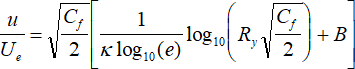
where, .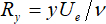

Given a series of C_f values, a family of curves can be generated for vs. R_y. Several values of R_y ranging from 100 to 100,000 and C_f values ranging from 0.001 to 0.006 should be used to plot the curves in a log-linear format. This forms the Clauser chart, which can be used to determine the skin friction coefficient, C_f, as shown in Figure 4. By comparing the measured boundary layer velocity profile with the family of curves that are based on the log law-of-the-wall with the prescribed skin-friction coefficient values, the curve that best overlaps with the log law portion of the measured velocity profile gives the value of the measured skin friction coefficient.

Figure 4: Clauser Chart.

This result can be compared to the result obtained using the integral equation method. Also, the velocity fluctuation profile can be obtained and the experimental result can be compared against the log law-of-the-wall. See the Appendix for more information.

The demonstration shows how to use constant temperature anemometry, a powerful tool used to study turbulent flow over a surface, which in this specific case was a flat plate. This method is simpler and less expensive than other methods, such as PIV, PTV, and LDV, and it provides a high temporal resolution. The application of hot-wire anemometry to a turbulent boundary layer provides a cost effective and hands-on approach to demonstrate the behavior of turbulent flows.

Constant temperature anemometry has numerous applications. This technique can be used to survey both turbulent and laminar flows. Hot-wire anemometry can be used to study the wake flows of an airfoil or an airplane model, thus providing information such as the drag of the airfoil and the level of wake turbulence, which provides valuable information for aircraft design.

Hot-wire anemometry can also be used in environmental fluid dynamics investigations, such as to study plume flows, which are responsible for the mass and momentum transport and mixing of a variety of processes found in the Earth`s atmosphere.

A variation to hot-wire anemometry is hot-film anemometry, which is typically used in liquid flows that require robust and reliable performance. For example, monitoring of the air flow at the air intake duct of an automobile engine is often performed by a sensor made of hot film.

The application of hotwire anemometry is not restricted to the mechanical engineering realm. CTA can also be used for example in biomedical applications to measure respiration rate.

Materials List

Name	Company	Catalog Number	Comments
Equipment
Instructional Subsonic Wind Tunnel	Jetstream		The dimensions of the test section of the wind tunnel are as follows: 5.25" (width) x 5.25"(height) x 16" (length). The wind tunnel should be able to attain air speeds of 0 - 80 mph.
The Wall			The wall of the test section is made of glass.
CTA model 1750	TSI Corp.
Hot-wire probe	TSI Corp	TSI 1218-T1.5	Tungsten-platinum coated, standard boundary layer probe. The diameter of the probe is 3.81 μm. The length of the sensing area of the wire is 1.27 mm.
A/D Board	National Instruments	NI USB 6003	Maximum sampling rate of 100 kHz with 16-bit resolution
Traverse System	Newport		Newport 370-RC Rack-And-Pinion Rod Clamp & 75 Damped Optical Support Rod Assembly
Pitot tube			The dynamic pressure of the free stream will be sensed by a tiny Pitot tube installed at the beginning region of the test section. The resolution of the Pitot tube is 0.1 mph.
Software			LabView software will be used for data acquisition.
Power Supply	Heath	2718	Heath 2718 Tri-Power Supply with 15V DC output is used to power the hot-wire anemometer.
Oscilloscope	Tektronix	2232
Signal Generator	Agilent	33110A