Characterization of Magnetic Components

Overview

Source: Ali Bazzi, Department of Electrical Engineering, University of Connecticut, Storrs, CT.

The objective of this experiment is to achieve hands-on experience with different magnetic components from design and material perspectives. This experiment covers B-H curves of magnetic material and inductor design through identifying unknown design factors. The B-H curve of a magnetic element, such as an inductor or transformer, is a characteristic of the magnetic material forming the core around which windings are wrapped. This characteristic provides information about the magnetic flux density that the core can handle with respect to the current flowing in the windings. It also provides information about limits before the core is magnetically saturated, i.e. when pushing more current through the coil leads to no further magnetic flux flow.

Principles

The B-H curve can be identified using a simple circuit. Using Ampere's law, the magnetic flux intensity (H) is proportional to the current in a coil; for example, for a single N-turn coil carrying a current (i) wrapped around a core of average length (l) and cross-sectional area (A), Ampere's law yields,

Equation 1 (1)

Also, the voltage across the coil (v) can be determined by the flux rate of change dφ/dt using Faraday's law. For the same coil described previously,

Equation 2 (2)

The flux density (B) is also defined as,

Equation 3 (3)

which can thus be written as,

Equation 4 (4)

Therefore, to estimate the B-H curve of a material, i and the time-integral of v can be used. Scaling back to the actual B and H quantities is possible when N, l, and A are known.

In order to measure the time-integral of v, a simple R-C circuit in parallel with the coil can be used (Fig. 1). The R-C divider should have R >> X_C at the operating frequency so that v_R≈v. Using this assumption, measuring the capacitor voltage v_C gives a reasonable approximation of the time integral of v since,

Equation 5 (5)

The negative sign is effective for time domain representation but should be dropped when dealing with RMS and peak quantities, thus it is common to use,

Equation 6 (6)

Figure 1: Test circuit to determine the B-H curve of an inductor. Please click here to view a larger version of this figure.

Procedure

1. Relative Permeability Identification

Follow the procedure to find the relative permeability of the small inductor (yellow/white ferrite core). The core dimensions are shown in Fig. 2, and the number of turns is N=75.

Using a LCR meter, measure the inductance of the inductor at both 120 Hz and 1000 Hz.
Build the circuit in Fig. 1 on a proto-board, but keep the function generator output disconnected from the proto-board.
Check a differential voltage probe and a current probe for no offsets with the current probe connected on channel 1 and the voltage probe connected on channel 2.
Note the scaling factors for the differential probe on the probe itself and on the scope. Set the differential probe to 1/20 for a better resolution.
Set the current probe to 100 mV/A on the probe itself and 1X on the scope. Remember that these scaling factors need to be used when performing calculations.
Set the function generator output (50 Ω BNC output connector) at 10 V peak and 1000 Hz sinusoidal waveform. Observe the waveform using the differential voltage probe.
Leave the function generator on even when disconnected, but avoid shorting its terminals. Turning the function generator off resets many settings.
Connect the current and voltage probes to measure v_C and i.
Check that the circuit is as desired and that all connections are maintained.
Connect the function generator to the circuit.
Take a screenshot of the measured current and voltage with at least three periods shown in addition to the peak or RMS values of the measured signals.
From the "Display" menu on the scope, change the display format from "YT" to "XY".
Observe the B-H curve by adjusting the channel 1 and channel 2 vertical adjustment knobs until the curve fits the scope screen.
In order to see a steadier curve, use the "persist" option from the display menu at a setting of 1 or 2 s.
Take a screenshot of the measured B-H curve.
Adjust the function generator frequency to 120 Hz and retake the B-H curve screenshot after adjusting the curve settings as needed.
Disconnect the function generator and remove the inductor. Keep the rest of the circuit intact.

Figure 2: Dimensions of the smaller inductor core. Please click here to view a larger version of this figure.

2. Identifying the Number of Turns

The larger black inductor (Bourns 1140-472K-RC) has an unknown number of turns. To simplify calculations, assume the core to be an all-air-core solenoid with a radius of 1.5 cm and length of 2.5 cm. If this assumption is not taken, the geometry of the core will have to be considered and will complicate calculations. However, this assumption is still reasonable given that with a solenoid, flux has to pass through air on both sides of the device and air is the dominant flux path medium.

Using the LCR meter, measure the inductance of the provided inductor at both 120 Hz and 1000 Hz.
Place the inductor in the circuit shown in Fig. 1 , which should still be intact from the previous part of the experiment.
Check a differential voltage probe and a current probe for no offsets with the current probe connected on channel 1 and the voltage probe connected on channel 2.
Note the scaling factors for the differential probe on the probe itself and on the scope. Set the differential probe to 1/20 for a better resolution.
Set the current probe to 100 mV/A on the probe itself and 1X on the scope. Remember that these scaling factors need to be used when doing calculations utilizing any measurements or data captures for further analysis.
Set the function generator output (50 Ω BNC output connector) at 10 V peak and 1000 Hz sinusoidal waveform. Observe the waveform using the differential voltage probe.
Leave the function generator on even when disconnected, but avoid shorting its terminals. Turning the function generator off resets many settings.
Connect the current and voltage probes to measure v_C and i.
Check the circuit, and make sure that connections are as desired.
Connect the function generator to the circuit.
Take a screenshot of the measured current and voltage with at least three periods shown in addition to the peak or RMS values of the measured signals.
From the "display" menu on the scope, change the display format from "YT" to "XY".
Observe the B-H curve by adjusting the channel 1 and channel 2 vertical adjustment knobs until the curve fits the scope screen.
In order to see a steadier curve, use the "persist" option from the display menu at a setting of 1 or 2 s.
Take a screenshot of the measured B-H curve.
Adjust the function generator frequency to 120 Hz and retake the B-H curve screenshot after adjusting the curve settings as needed.
Turn off the function generator and disassemble the circuit.

3. B-H Curve of a 60 Hz Transformer

The transformer used in this demonstration steps down 115 V RMS to 24 V RMS, but can only be used for B-H curve characterization in this experiment, thus only the 120 V RMS terminals are used. The transformer dimensions are shown in Fig. 3.

Using the LCR meter, measure the inductance of the 115 V-side winding at 120 Hz (closer to the rated 60 Hz).
Make sure the three-phase disconnect switch is in the off position.
Connect the three-phase cable to the VARIAC.
Build the circuit shown in Fig. 4. Have the transformer sit on the side of the proto-board. Use banana cables to connect AC1 and N from the VARIAC to the proto-board.
Make sure the VARIAC is set at 0%.
Check a differential voltage probe and a current probe for no offsets with the current probe connected on channel 1 and the voltage probe connected on channel 2.
Note down the scaling factors for the differential probe on the probe itself and on the scope. Set the differential probe scaling to 1/200.
Set the current probe to 100 mV/A on the probe itself and 1X on the scope. Remember that these scaling factors need to be used when doing calculations.
Connect the current and voltage probes to measure v_C and i.
Check the circuit.
Turn on the three-phase disconnect switch, and slowly adjust the VARIAC until 90% is reached.
Take a screenshot of the measured current and voltage with at least three periods shown in addition to the peak or RMS values of the measured signals.
From the "Display" menu on the scope, change the display format from "YT" to "XY".
Observe the B-H curve by adjusting the channel 1 and channel 2 vertical adjustment knobs until the curve fits the scope screen.
In order to see a steadier curve, use the "persist" option from the display menu at a setting of 1 or 2 s.
Take a screenshot of the measured B-H curve.
Restore the VARIAC to 0%, turn the disconnect switch off, and disassemble the circuit.

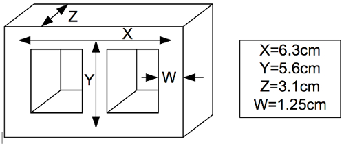
Figure 3: Dimensions of the transformer core. Please click here to view a larger version of this figure.

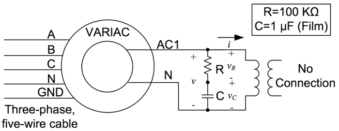
Figure 4: Test circuit to determine the B-H curve of a 60 Hz transformer. Please click here to view a larger version of this figure.

Results

In order to find the relative permeability of the core material, two approaches can be used. The first approach is to use an LCR meter, where the inductance (L) of a coil made with a known number of turns (N) is measured, and then the relative permeability can be calculated as follows:

Reluctance of the core: Equation 7 (7)

The relative permeability (µ_r) is thus:

Equation 8 (8)

where µ_o is the permeability of vacuum, l is the average core length in m, and A is the core cross-sectional area in m².

For example, if a toroidal core is used with an internal radius r₁=1 cm, an external radius r₂=2 cm, a cross-sectional area of 1 cm², and the LCR meter reads 1 µH for 10 turns, then:

l=2π(r₂-r₁) =2π cm, 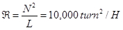Equation 9 , and µ_r=50,000.

The second method uses the measured B-H curve. In the linear region, which is either visible or approximated, the relative permeability can be found from the slope (B=µ_rµ_oH) for each frequency. To find B and H values, appropriate scaling should be performed for probe factors, circuit elements, and core dimensions using previous measurements.

In an approach similar to finding the relative permeability, the number of turns can be found if the relative permeability is unknown. This can be achieved by manipulating the previous equations to find N.

For ferrites, µ_ris on the order of several thousands, while for steel and steel alloys, µ_ris on the order of tens or hundreds.

Application and Summary

Even though inductors and other electro-magnetic devices (e.g., transformers) are very common in many electrical, electronic, and mechanical systems, buying inductors for a specific application is not trivial. Even when an inductor is bought, datasheet information may still have ambiguities on the actual material, number of turns, and other details. The tests in this experiment are especially useful for engineers and technicians who plan to build their own inductors or characterize off-the-shelf ones. This is common with power electronics applications (e.g., DC/DC converters) as well as electric motor drive applications (e.g., AC filter inductors) where more information is desired about the inductor in hand.

Tags

Magnetic Components Inductors Transformers Magnetic Material Core Coil Current Flow Magnetic Field Permeability Magnetizing Force Magnetic Flux B H Curve Magnetic Saturation Measurement Characterization Windings Flux Density Hysteresis

1. Relative Permeability Identification

Follow the procedure to find the relative permeability of the small inductor (yellow/white ferrite core). The core dimensions are shown in Fig. 2, and the number of turns is N=75.

Using a LCR meter, measure the inductance of the inductor at both 120 Hz and 1000 Hz.
Build the circuit in Fig. 1 on a proto-board, but keep the function generator output disconnected from the proto-board.
Check a differential voltage probe and a current probe for no offsets with the current probe connected on channel 1 and the voltage probe connected on channel 2.
Note the scaling factors for the differential probe on the probe itself and on the scope. Set the differential probe to 1/20 for a better resolution.
Set the current probe to 100 mV/A on the probe itself and 1X on the scope. Remember that these scaling factors need to be used when performing calculations.
Set the function generator output (50 Ω BNC output connector) at 10 V peak and 1000 Hz sinusoidal waveform. Observe the waveform using the differential voltage probe.
Leave the function generator on even when disconnected, but avoid shorting its terminals. Turning the function generator off resets many settings.
Connect the current and voltage probes to measure v_C and i.
Check that the circuit is as desired and that all connections are maintained.
Connect the function generator to the circuit.
Take a screenshot of the measured current and voltage with at least three periods shown in addition to the peak or RMS values of the measured signals.
From the "Display" menu on the scope, change the display format from "YT" to "XY".
Observe the B-H curve by adjusting the channel 1 and channel 2 vertical adjustment knobs until the curve fits the scope screen.
In order to see a steadier curve, use the "persist" option from the display menu at a setting of 1 or 2 s.
Take a screenshot of the measured B-H curve.
Adjust the function generator frequency to 120 Hz and retake the B-H curve screenshot after adjusting the curve settings as needed.
Disconnect the function generator and remove the inductor. Keep the rest of the circuit intact.

Figure 2: Dimensions of the smaller inductor core. Please click here to view a larger version of this figure.

2. Identifying the Number of Turns

The larger black inductor (Bourns 1140-472K-RC) has an unknown number of turns. To simplify calculations, assume the core to be an all-air-core solenoid with a radius of 1.5 cm and length of 2.5 cm. If this assumption is not taken, the geometry of the core will have to be considered and will complicate calculations. However, this assumption is still reasonable given that with a solenoid, flux has to pass through air on both sides of the device and air is the dominant flux path medium.

Using the LCR meter, measure the inductance of the provided inductor at both 120 Hz and 1000 Hz.
Place the inductor in the circuit shown in Fig. 1 , which should still be intact from the previous part of the experiment.
Check a differential voltage probe and a current probe for no offsets with the current probe connected on channel 1 and the voltage probe connected on channel 2.
Note the scaling factors for the differential probe on the probe itself and on the scope. Set the differential probe to 1/20 for a better resolution.
Set the current probe to 100 mV/A on the probe itself and 1X on the scope. Remember that these scaling factors need to be used when doing calculations utilizing any measurements or data captures for further analysis.
Set the function generator output (50 Ω BNC output connector) at 10 V peak and 1000 Hz sinusoidal waveform. Observe the waveform using the differential voltage probe.
Leave the function generator on even when disconnected, but avoid shorting its terminals. Turning the function generator off resets many settings.
Connect the current and voltage probes to measure v_C and i.
Check the circuit, and make sure that connections are as desired.
Connect the function generator to the circuit.
Take a screenshot of the measured current and voltage with at least three periods shown in addition to the peak or RMS values of the measured signals.
From the "display" menu on the scope, change the display format from "YT" to "XY".
Observe the B-H curve by adjusting the channel 1 and channel 2 vertical adjustment knobs until the curve fits the scope screen.
In order to see a steadier curve, use the "persist" option from the display menu at a setting of 1 or 2 s.
Take a screenshot of the measured B-H curve.
Adjust the function generator frequency to 120 Hz and retake the B-H curve screenshot after adjusting the curve settings as needed.
Turn off the function generator and disassemble the circuit.

3. B-H Curve of a 60 Hz Transformer

The transformer used in this demonstration steps down 115 V RMS to 24 V RMS, but can only be used for B-H curve characterization in this experiment, thus only the 120 V RMS terminals are used. The transformer dimensions are shown in Fig. 3.

Using the LCR meter, measure the inductance of the 115 V-side winding at 120 Hz (closer to the rated 60 Hz).
Make sure the three-phase disconnect switch is in the off position.
Connect the three-phase cable to the VARIAC.
Build the circuit shown in Fig. 4. Have the transformer sit on the side of the proto-board. Use banana cables to connect AC1 and N from the VARIAC to the proto-board.
Make sure the VARIAC is set at 0%.
Check a differential voltage probe and a current probe for no offsets with the current probe connected on channel 1 and the voltage probe connected on channel 2.
Note down the scaling factors for the differential probe on the probe itself and on the scope. Set the differential probe scaling to 1/200.
Set the current probe to 100 mV/A on the probe itself and 1X on the scope. Remember that these scaling factors need to be used when doing calculations.
Connect the current and voltage probes to measure v_C and i.
Check the circuit.
Turn on the three-phase disconnect switch, and slowly adjust the VARIAC until 90% is reached.
Take a screenshot of the measured current and voltage with at least three periods shown in addition to the peak or RMS values of the measured signals.
From the "Display" menu on the scope, change the display format from "YT" to "XY".
Observe the B-H curve by adjusting the channel 1 and channel 2 vertical adjustment knobs until the curve fits the scope screen.
In order to see a steadier curve, use the "persist" option from the display menu at a setting of 1 or 2 s.
Take a screenshot of the measured B-H curve.
Restore the VARIAC to 0%, turn the disconnect switch off, and disassemble the circuit.

Figure 3: Dimensions of the transformer core. Please click here to view a larger version of this figure.

Figure 4: Test circuit to determine the B-H curve of a 60 Hz transformer. Please click here to view a larger version of this figure.

Skip to...

0:06

Overview

1:21

Principles of Magnetic Component Characterization

4:04

Measuring Relative Permeability

6:12

Identifying the Number of Turns

7:08

B-H Curve of a 60 Hz Transformer

8:04

Representative Results

8:50

Applications

10:15

Summary

Videos from this collection:

article

Now Playing

Characterization of Magnetic Components

Electrical Engineering

15.0K Views

article

Electrical Safety Precautions and Basic Equipment

Electrical Engineering

144.6K Views

article

Introduction to the Power Pole Board

Electrical Engineering

12.4K Views

article

DC/DC Boost Converter

Electrical Engineering

56.8K Views

article

DC/DC Buck Converter

Electrical Engineering

21.1K Views

article

Flyback Converter

Electrical Engineering

13.2K Views

article

Single Phase Transformers

Electrical Engineering

20.1K Views

article

Single Phase Rectifiers

Electrical Engineering

23.4K Views

article

Thyristor Rectifier

Electrical Engineering

17.5K Views

article

Single Phase Inverter

Electrical Engineering

17.9K Views

article

DC Motors

Electrical Engineering

23.3K Views

article

AC Induction Motor Characterization

Electrical Engineering

11.6K Views

article

VFD-fed AC Induction Machine

Electrical Engineering

6.9K Views

article

AC Synchronous Machine Synchronization

Electrical Engineering

21.6K Views

article

AC Synchronous Machine Characterization

Electrical Engineering

14.2K Views

Copyright © 2025 MyJoVE Corporation. All rights reserved