The Evans Method
Обзор
Source: Tamara M. Powers, Department of Chemistry, Texas A&M University
While most organic molecules are diamagnetic, wherein all their electrons are paired up in bonds, many transition metal complexes are paramagnetic, which has ground states with unpaired electrons. Recall Hund's rule, which states that for orbitals of similar energies, electrons will fill the orbitals to maximize the number of unpaired electrons before pairing up. Transition metals have partially populated d-orbitals whose energies are perturbed to varying extents by coordination of ligands to the metal. Thus, the d-orbitals are similar in energy to one another, but are not all degenerate. This allows for complexes to be diamagnetic, with all electrons paired up, or paramagnetic, with unpaired electrons.
Knowing the number of unpaired electrons in a metal complex can provide clues into the oxidation-state and geometry of the metal complex, as well as into the ligand field (crystal field) strength of the ligands. These properties greatly impact the spectroscopy and reactivity of transition metal complexes, and so are important to understand.
One way to count the number of unpaired electrons is to measure the magnetic susceptibility, χ, of the coordination compound. Magnetic susceptibility is the measure of magnetization of a material (or compound) when placed in an applied magnetic field. Paired electrons are slightly repelled by an applied magnetic field, and this repulsion increases linearly as the strength of the magnetic field increases. On the other hand, unpaired electrons are attracted (to a larger extent) to a magnetic field, and the attraction increases linearly with magnetic field strength. Therefore, any compound with unpaired electrons will be attracted to a magnetic field.1
When we measure the magnetic susceptibility, we obtain information on the number of unpaired electrons from the magnetic moment, µ. The magnetic susceptibility is related to the magnetic moment, µ by Equation 12:
 (1)
(1)
The constant  = [(3kB)/Nβ2)], where β= Bohr magneton of the electron (0.93 x 10⁻²⁰ erg gauss-1), N = Avogadro's number, and kB = Boltzmann constant
XM = molar magnetic susceptibility (cm3/mol)
T = temperature (K)
µ = magnetic moment, measured in units of Bohr magneton, µB = 9.27 x 10⁻²⁴ JT-1
The magnetic moment for complexes is given by Equation 21:
 (2)
(2)
g = gyromagnetic ratio = 2.00023 µB
S = spin quantum number = ∑ms = [number of unpaired electrons, n]/2
L = orbital quantum number = ∑ml
This equation has both orbital and spin contributions. For first-row transition metal complexes, the orbital contribution is small and hence can be omitted, so the spin-only magnetic moment is given by Equation 3:
 (3)
(3)
The spin-only magnetic moment can thus directly give the number of unpaired electrons. This approximation can also be made for heavier metals, though orbital contributions may be significant for second and third row transition metals. This contribution may be so significant that it inflates the magnetic moment enough that the compound appears to have more unpaired electrons than it does. Therefore, additional characterization may be required for these complexes.
In this experiment, the solution magnetic moment of tris(acetylacetonato)iron(III) (Fe(acac)3) is determined experimentally using Evans method in chloroform.
Принципы
There are many methods to measure the magnetic susceptibility. In the late 19th century, Louis Georges Gouy developed the Gouy balance, which is a highly accurate method to measure magnetic susceptibility. In this approach, an analytic balance is used to mass a magnet, and the change in mass observed upon placing a paramagnetic sample between the poles of the magnet is related to the magnetic susceptibility. This method is not practical, as suspending the sample between the poles of the magnet is not trivial. This requires four measurements of mass between which the magnet cannot move, and for air-sensitive samples, this measurement must be conducted within a glovebox. More modern magnetic susceptibility balances are available, but this requires the purchase of such a balance.
Another method is to use a SQUID (Superconducting Quantum Interference Device) magnetometer. This requires several mg of solid sample, and unless other magnetic measurements are to be done on the sample, is not practical or cost-effective for paramagnetic complexes that can be made into solutions.
Finally, and what will be demonstrated here, is the use of an NMR spectrometer to measure the magnetic susceptibility. This approach was developed by Dennis Evans in 1959. It is simple and relies on the effect a paramagnet in solution has on the chemical shift of a reference compound, usually the solvent. Data collection can be done on any NMR spectrometer, the data is easy to interpret, and sample preparation is straightforward and requires little material. It has become the standard method to obtain magnetic susceptibility data for inorganic complexes.
The measurement of magnetic susceptibility by the Evans method relies on the fact that the unpaired electrons from the paramagnet in solution will result in a change of the chemical shift of all species in solution (Figure 1). Thus, by noting the chemical shift difference of a solvent molecule in the presence and absence of a paramagnetic species, the magnetic susceptibility can be obtained via Equation 4 (for a high-field NMR spectrometer)3
 (4)
(4)
Δf = frequency difference in Hz between the shifted resonance and the pure solvent resonance
F = spectrometer radiofrequency in Hz
c = concentration of paramagnetic species (mol/mL)
Data is readily obtained by collecting a 1H NMR spectrum of a sample that contains a capillary of pure solvent, with a solution of the paramagnet surrounding the capillary within the NMR tube (Figure 2).

Figure 1. Example 1H NMR spectrum of the experiment
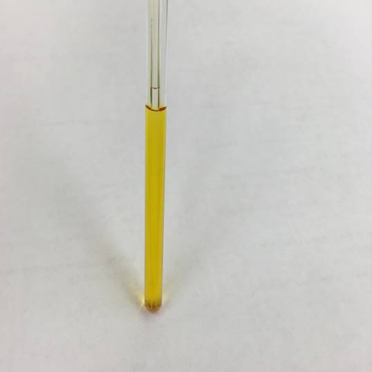
Figure 2. Image of a capillary in NMR tube setup
Процедура
1. Preparation of Capillary Insert
- Using a lighter or other gas flame, melt the tip of a long Pasteur pipette. Gently rotate the pipette tip in the flame until a small bulb forms. Allow the glass to cool.
- In a scintillation vial, prepare a 50:1 (volume) solution of deuterated:proteo chloroform. Pipette 2 mL of deuterated solvent, and to this add 40 µL of proteo solvent. Cap the vial.
- Carefully add a few drops of the solvent mixture to the sealed glass pipette. Gently flick the tip of the sealed pipette so that the liquid enters the capillary. Repeat until the solution has a depth of ~ 2 inches from the bottom of the capillary. Make sure that there are no bubbles of air.
- Cap the pipette with a 14/20 rubber septum. Using a 3-mL syringe capped with a needle, insert the needle into the pipette and pull out 3 mL of air. This creates a partial vacuum, facilitating the next step.
- Seal the top of the capillary. Horizontally clamp the pipette to a ring stand. Use a lighter to soften the glass above the solution in the bottom of the pipette. Once the glass softens, begin to rotate the tip of the pipette and pull the tip of the pipette away from the clamped base. Let the sealed capillary cool.
2. Preparation of Paramagnetic Solution
- Using an analytical balance, mass a scintillation vial and lid. Note the mass.
- Mass out 5-10 mg of the Fe(acac)3 in the scintillation vial, and note the mass. Fe(acac)3 has a very high solution magnetic moment. Therefore 5-10 mg will generate a large change of the chemical shift. Typically, 10 - 15 mg is a more appropriate mass to use for Evans method samples.
- Pipette ~600 µL of the prepared solvent mixture into the vial containing the paramagnetic species. Cap the vial, and note the mass. Make sure that the solid completely dissolves.
3. Preparation of NMR Sample
- In a standard NMR tube, carefully drop the capillary insert at an angle, to ensure it does not break it.
- Pipette in the solution containing the paramagnetic species.
- Cap the NMR tube. For air-sensitive samples, wrap Parafilm around the cap.
4. Data Collection
- Acquire and save a standard 1H NMR spectrum.
- Note the temperature of the probe.
- Note the radiofrequency.
5. Data Analysis and Results
- Using the mass and density of the solvent, calculate the volume of the solvent used to prepare the paramagnetic solution.
- Calculate the concentration (M) of the paramagnetic solution.
- Calculate the peak separation of the solvent resonance between that of pure solvent (in the capillary) and that shifted by the paramagnet (outside of the capillary) (Δppm). If this is done in ppm, convert it to Hz by Equation 5:
 (5)
(5)
F = spectrometer radiofrequency in Hz - Calculate the magnetic susceptibility using Equation 4.
- Calculate the magnetic moment using Equation 1.
- Compare the magnetic moment obtained with that predicted for n unpaired electrons from Equation 3. The magnetic susceptibility will be slightly greater than the anticipated spin-only value given in the table, but should be less than that which corresponds to n+1 unpaired electrons.
- Give the number of unpaired electrons for the paramagnetic species.
6. Troubleshooting
- If two well-resolved solvent peaks are not observed, try the following:
- Use a spectrometer with a greater field strength to increase the chemical shift difference (in ppm) of the two peaks.
- Make the sample more concentrated, so that the shift is larger.
- Sometimes the value does not make sense. If a value that is too low is obtained, try the following:
- Repeat, taking greater care in massing out the solvent and paramagnetic species.
- Make sure that the paramagnetic species being used is pure. Even solvent impurities in crystals will affect the mass and hence concentration.
- For large molecules, the diamagnetism may be so significant that a diamagnetic correction must be made. This term is subtracted to Equation 4:

- Sometimes the value does not make sense. If a value that is too high is obtained, try the following:
- Follow the same steps as 6.2.1-6.2.3.
- For heavier metals, inclusion of orbital contributions may be necessary.
7. Air-sensitive Samples
- Air-sensitive samples can readily be analyzed using this technique. Steps 1.2-1.4, step 2, and step 3 are simply performed inside a glove-box.
Результаты
Experimental Results
| Fe(acac)3 | Chloroform | |
| m (g) | 0.0051 | 0.874 |
| MW (g/mol) | 353.17 | n/a |
| n (mol) | 1.44⋅10-5 | n/a |
| Density (g/mL) | n/a | 1.49* |
| Volume (mL) | n/a | 0.587 |
| c (mol/mL) | 2.45⋅10-5 | |
| NMR shifts | Peak 1 | Peak 2 |
| δ (ppm) | 7.26 | 5.85 |
| Δppm | 1.41 | |
| NMR Instrument | ||
| Temperature (K) | 296.3 | |
| Field, F (Hz) | 500⋅106 |
* the density of the solvent can be approximated to the density of the solvent used
Calculations:

 = 0.0137 cm3/mol
 = 5.70 µB
Theoretical Results for Given S and n Values:
| S | n | μS |
| 1/2 | 1 | 1.73 |
| 1 | 2 | 2.83 |
| 3/2 | 3 | 3.87 |
| 2 | 4 | 4.90 |
| 5/2 | 5 | 5.92 |
For 4.5 mg of Fe(acac)3 dissolved in 0.58 mL solvent, with a 300 MHz instrument a peak separation of 1.41 ppm is observed, which gives XM= 1.37 x 10⁻² and µeff = 5.70. This µeff value is consistent with an S = 5/2 complex, which has 5 unpaired electrons.
Заявка и Краткое содержание
The Evans method is a simple and practical method for obtaining the magnetic susceptibility of soluble metal complexes. This provides the number of unpaired electrons in a metal complex, which is pertinent to the spectroscopy, magnetic properties, and reactivity of the complex.
Measuring the magnetic susceptibility of paramagnetic species gives the number of unpaired electrons, which is a key property of metal complexes. As the reactivity of metal complexes is influenced by its electronic structure - that is, how the d-orbitals are populated - it is important to establish the number of unpaired electrons. The magnetic susceptibility can be used to determine the geometry of the metal complex in solution, give insight into the ligand field strength, and can provide evidence for the correct formal oxidation-state assignment of the metal complex. In the modules on "Group Theory" and "MO Theory of Transition Metal Complexes," we will introduce how to predict d-orbital splitting diagrams as well as how to use data from the Evans method to help determine the geometry of a metal complex and provide evidence for the oxidation state of the metal center.
There are multiple instruments that can be used to measure the magnetic susceptibility of a paramagnetic species including a Gouy balance, SQUID, or NMR instrument. The Evans method is a simple and practical technique that uses NMR to determine the solution magnetic moment of a paramagnet. While the Evans method is a powerful tool in the field of magnetism, there are several drawbacks to the technique. First, the molecule must be soluble in the solvent used in the experiment. If the paramagnetic sample is not fully dissolved, the concentration of the solution will be incorrect, which will lead to errors in the experimentally determined solution magnetic moment. Other errors in concentration can arise if the paramagnetic sample has diamagnetic (solvent) or paramagnetic impurities.
Ссылки
- Miessler, G. L., Fischer, P. J., Tarr, D. A. Inorganic Chemistry. 5 ed. Pearson. (2014).
- Drago, R. S. Physical Methods for Chemists. 2 ed. Saunders College Publishing. (1992).
- Girolami, G. S., Rauchfuss, T. B., Angelici, R. J. Synthesis and Technique in Inorganic Chemistry: A Laboratory Manual. 3 ed. University Science Books. Sausalito, CA, (1999).
Перейти к...
Видео из этой коллекции:

Now Playing
The Evans Method
Inorganic Chemistry
68.0K Просмотры

Synthesis Of A Ti(III) Metallocene Using Schlenk Line Technique
Inorganic Chemistry
31.5K Просмотры

Glovebox and Impurity Sensors
Inorganic Chemistry
18.6K Просмотры

Purification of Ferrocene by Sublimation
Inorganic Chemistry
54.3K Просмотры

Single Crystal and Powder X-ray Diffraction
Inorganic Chemistry
104.0K Просмотры

Electron Paramagnetic Resonance (EPR) Spectroscopy
Inorganic Chemistry
25.4K Просмотры

Mössbauer Spectroscopy
Inorganic Chemistry
21.9K Просмотры

Lewis Acid-Base Interaction in Ph3P-BH3
Inorganic Chemistry
38.7K Просмотры

Structure Of Ferrocene
Inorganic Chemistry
79.1K Просмотры

Application of Group Theory to IR Spectroscopy
Inorganic Chemistry
45.0K Просмотры

Molecular Orbital (MO) Theory
Inorganic Chemistry
35.1K Просмотры

Quadruply Metal-Metal Bonded Paddlewheels
Inorganic Chemistry
15.3K Просмотры

Dye-sensitized Solar Cells
Inorganic Chemistry
15.7K Просмотры

Synthesis of an Oxygen-Carrying Cobalt(II) Complex
Inorganic Chemistry
51.5K Просмотры

Photochemical Initiation Of Radical Polymerization Reactions
Inorganic Chemistry
16.7K Просмотры
Авторские права © 2025 MyJoVE Corporation. Все права защищены