Computational Fluid Dynamics Simulations of Blood Flow in a Cerebral Aneurysm

Source: Joseph C. Muskat, Vitaliy L. Rayz, and Craig J. Goergen, Weldon School of Biomedical Engineering, Purdue University, West Lafayette, Indiana

The objective of this video is to describe recent advancements of computational fluid dynamic (CFD) simulations based on patient- or animal-specific vasculature. Here, subject-based vessel segmentations were created, and, using a combination of open-source and commercial tools, a high-resolution numerical solution was determined within a flow model. Numerous studies have demonstrated that the hemodynamic conditions within the vasculature affect the development and progression of atherosclerosis, aneurysms, and other peripheral artery diseases; concomitantly, direct measurements of intraluminal pressure, wall shear stress (WSS), and particle residence time (PRT) are difficult to acquire in vivo.

CFD allow such variables to be assessed non-invasively. In addition, CFD is used to simulate surgical techniques, which provides physicians better foresight regarding post-operative flow conditions. Two methods in magnetic resonance imaging (MRI), magnetic resonance angiography (MRA) with either time of flight (TOF-MRA) or contrast-enhanced MRA (CE-MRA) and phase-contrast (PC-MRI), allow us to obtain vessel geometries and time-resolved 3D velocity fields, respectively. TOF-MRA is based on the suppression of the signal from static tissue by repeated RF pulses that are applied to the imaged volume. A signal is obtained from unsaturated spins moving into the volume with the flowing blood. CE-MRA is a better technique for imaging vessels with complex recirculating flows, as it uses a contrast agent, such as gadolinium, to increase the signal.

Separately, PC-MRI utilizes bipolar gradients to generate phase shifts that are proportional to a fluid's velocity, thus providing time-resolved velocity distributions. While PC-MRI is capable of providing blood flow velocities, the accuracy of this method is affected by limited spatiotemporal resolution and velocity dynamic range. CFD provides superior resolution and can assess the range of velocities from high-speed jets to slow recirculating vortices observed in diseased blood vessels. Thus, even though the reliability of CFD depends on the modeling assumptions, it opens up the possibility for high quality, comprehensive depiction of patient-specific flow fields, which can guide diagnosis and treatment.

TOF-MRA, CE-MRA and PC-MRI are often used as input geometry and flow boundary conditions for CFD simulations. As discussed above, vessel geometry and inflow boundary conditions (velocity profiles through a cross-section) are measured for each subject. For the data included in this study, the TOF-MRA resolution was 0.26 x 0.26 x 0.50 mm, while the PC-MRI resolution was 1.00 x 1.00 x 1.20 mm. The 4D Flow MRI sequence was used to acquire the three-dimensional velocity distribution through the cardiac cycle. The TOF data is segmented pseudo-automatically with a variety of tools. The image resolution, i.e., the size of a voxel, directly influences the quality of the resulting model of the geometry. 4D Flow MRI determines the velocity  of blood at each voxel using phase shift according to the following equations:

(1)

(2)

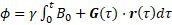
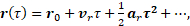
Measured phase shifts and velocities depend on the gradient field , the gyromagnetic ratio , the initial position of the spin , the spin velocity , and the spin acceleration . The magnetic fields and material constants are defined while initializing the MRI scan. 4D Flow MRI encodes in three orthogonal directions to obtain three-dimensional velocity fields. Then, 3D models for each patient- or animal-specific case can be generated. The methods detailed in the procedure section will bring us to a CFD simulation by numerically solving the Navier-Stokes equations, which are generalized as:

₍₃₎

where is density, is flow velocity, p is pressure, and mu is the dynamic viscosity of the flow.

A precursor to the tutorial is the creation of a patient-specific vasculature model. In this demonstration, the tools Materialise Mimics, 3D Systems Geomagic Design X, and Altair HyperMesh were used to generate a tetrahedral volume mesh from MRA data.

1. Generate vessel centerlines for the model

1. Open the vmtk-launcher python GUI. In the PypePad, type: vmtkcenterlines -ifile [STL file saved to desktop].stl -ofile [STL name]centerlines.vtp
2. Select Run, Run all to load the data into the program. A new window will open that displays instructions and a rendering of the input model. Rotate the model and place the curser on each inlet location. Press the spacebar to place a seed.
3. After placing seeds on all of the inlets, press 'Q' to continue. Repeat the same placement of seeds for all outlets. After placing the outlet seeds, press 'Q' again and let the program run. This will save the centerline file to the desktop.

2. Data set-up in visualization software

1. Start the open-source visualization tool, ParaView (version 5.4.1 used in this procedure).
2. Select File, Open…, and locate the previously created files: the patient-specific volume mesh, centerline file(s), and the EnSight.case file(s). After clicking Ok, all data should be loaded into the interface.
3. From the bottom-left Properties table, select Apply. This command will load and read all the information a user has loaded or changed in ParaView. Highlight the volume mesh by clicking on its name within the Pipeline Browser to activate this selection.
4. Again, in the Properties table, scroll and change the Opacity value to somewhere between 0.2 - 0.5. Now, the centerlines and geometry renderings should be visible.

3. Remap 4D Flow MRI data with the volumetric mesh-grid and delete noise

1. From the top menu, select Filters, Alphabetical, ResampleWithDataset. A new window will open. Set the Source as the volume mesh and the Input as the EnSight.case file. Select Ok once these are set.
2. In the Properties table, select Apply to apply the filter.
3. As before, highlight the new ResampleWithDataset# name to activate it. Reduce the opacity of this new rendering as mentioned previously. In addition, change the centerline(s) from Surface to Points in the top menu.

4. Determine inlet and outlet flow boundary conditions

1. On the right side of the interface, next to maximize and minimize rendering options, select the Create View tool (square with vertical line). Select the SpreadSheet View option.
2. From the Showing dropdown box, select the centerline file(s). Only one type of file can be selected at a time. Cycle through the data, selecting various points to identify a location within each inlet and outlet.
3. Now, use the SpreadSheet View underneath Points to calculate the normal vector between two points near the same locations found in (4.2).
4. After finding the normal vector for each inlet and outlet locations, select Filters, Alphabetical, Slice. Make sure to activate the ResampleWithDataset# beforehand.
5. The Slice filter needs to appear beneath a new branch coming from ResampleWithDataset#. In the Properties table, set the plane Origin as the same XYZ point location for one of the two points used to calculate the normal vector. Use the normal vector from (4.3) to fill out the Normal values. Select Apply.
6. Highlight/activate the Slice# filter just created, and select Filters, Alphabetical, Surface Flow, and then Apply. Activate the new SurfaceFlow# item in the Pipeline Browser, and apply the Filters, Alphabetical, Group Time Steps, Apply.
7. In SpreadSheet View, open the GroupTimeSteps# data. Export this data to Microsoft Excel through copy and paste or use Export Spreadsheet.
8. In Excel, calculate the weighted values corresponding to the ratio of the flow rate at each outlet to the total inlet flow rate. Due to inherent noise and error of the 4D Flow MRI data, identify the smallest (generally having less reliable data) vessel to leave "open" to ensure the conservation of mass.
9. In CFD simulation software, transient flow waveforms are imported using read-transient-tables command; therefore, save the inlet flow data in a compatible, .txt format described in the online tutorials.

5. Set-up CFD simulations

1. Open CFD simulation software. Here we use ANSYS Fluent (version 18.1 described in this procedure as default). Choose File, Read, and Case…, and open the volume mesh .cas file used previously in ParaView. Display the mesh (this procedure uses a .cas file generated with Altair HyperMesh) by selecting Display…, Display.
2. It is importnat to scale the geometry to ensure the correct physical size of the model. Select Scale… and apply whatever unit conversion is necessary for the specific case then Close.
3. Select Materials, Create/Edit  to enter the material properties for blood. This tutorial uses physiologically relevant values of 1060 kg/s and 0.0035 kg/ms for density and viscosity, respectively.
4. Set the transient flow Boundary Conditions by prescribing either mass flow or velocity flow rates as a function of time for each inlet. Use the waveforms obtained from 4D Flow MRI measurement to prescribe the inlet boundary conditions. Outlets are given weighted values found in (4.8).
5. Under Solution, Methods, set the numerical schemes used for spatial and temporal discretization of the Navier-Stokes equations. For this procedure, use Coupled, which enables full pressure-velocity coupling, Least Squares Cell Based (gradient), Second Order scheme for pressure, Third-Order MUSCL scheme for momentum equations, and Second Order Implicit scheme for discretization in time. Ensure that the Time parameter in the top left has been set to Transient.
6. Under Solution, Initialization, select Standard Initialization. With all Initial Values set to 0, select Initialize. Now the program is set to run. Designate a solution folder to save results every Autosave Every (Time Steps) underneath Calculation Activities.
7. In the final steps, set-up the Time Step Size(s) under Run Calculation. Use the Excel boundary condition data in (4.7) to determine this value. Reducing the time step facilitates convergence and improves the accuracy of the numerical solution, while increasing the solution time. It is a good practice to run the simulation for at least three full cardiac cycles to eliminate the effect of the initial transients.
8. Finally, set Max Iterations for each time step between 300 - 500. The software will automatically stop the iterations at each time step once the convergence is reached and proceed to the following time step. The convergence can be improved by running a steady flow simulation with averaged velocity values and then using the results as the initial conditions for the pulsatile flow simulation. Select Calculate when ready to run the solver.
9. The software will run each iteration until convergence is achieved or Max Iterations causes the iteration to continue. The files will be automatically saved in the location from (5.5), and the solution data can be visualized in either ANSYS CFD-Post or ParaView software.

In this demonstration, a subject-specific model of a cerebral aneurysm was generated and the CFD was used to simulate the flow field. By providing detailed flow features and quantifying hemodynamics forces not obtainable from imaging data, CFD can be used to augment lower resolution 4D Flow MRI data.  Figure 1 shows how CFD gives a more complete description of the flow in the near-wall, re-circulating regions.

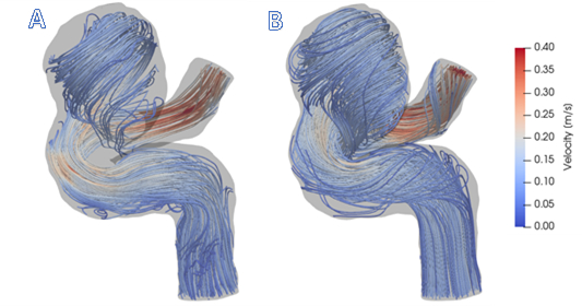
Figure 1: A) Visualization of 4D Flow MRI data within the vessel geometry. B) Visualization of CFD simulation results. In general, CFD streamlines give fuller understanding of blood flow patterns within this cerebral aneurysm.

Figure 1 shows that CFD results are in agreement with in vivo 4D Flow MRI. Figure 1 (A) shows the complex, recirculating flow patterns within the aneurysmal region, the balloon-like dilatation of the artery, which were detected with 4D Flow MRI. However, regions of stagnant flow in the top and bottom sections of the lesion are not filled with streamlines. This is because the signal to noise ratio in these regions is low. CFD-simulated flow, shown in Figure 1 (B), provides a higher resolution velocity field, particularly near the vessel walls. Thus, CFD models are capable of providing higher accuracy estimates of clinically-relevant, flow-derived metrics, such as pressure, WSS, and PRT, which can be used to predict aneurysmal disease progression.

Additionally, CFD simulations can be used to model postoperative flow conditions that would result from alternative treatment options. For example, Figure 2 (A) and (B) compare flow through the same vessel with different inflow rates. By prescribing varied boundary conditions, such as simulating vessel occlusion with no flow, the flow after a variety of surgical treatments is shown.

Figure 2: A) Simulation for surgical clipping of the right anterior cerebral artery (ACA). B) Simulation for surgical clipping of the left ACA. For simplicity, this figure maintains the preoperative inflow rate at the non-modified inlet; in reality, the flow rate would increase in the open vessel to compensate. C) Normal blood flow rates prescribe the inlet conditions for this model. Patient data from 4D Flow MRI provide inlet conditions for realistic visualization of flow patterns.

The ability to simulate postoperative flow fields resulting from various surgical treatments is an important advantage of CFD models. By applying realistic, patient-specific geometries and inflow data, different treatment scenarios can be demonstrated to provide physicians with information on the effect of a planned procedure on flow patterns. For example, Figure 2 (A) and (B) show recirculating flows that would occur if one or the other proximal artery is clipped. Treatments such as vessel clipping or deploying a flow diverter can be simulated, allowing physicians and patients to decide what will work best in each specific case.

The framework described here can be used to perform patient-specific CFD simulations. A high-resolution mesh is used to interpolate low-resolution 4D Flow MRI data; this isolates the flow data and minimizes error associated with noise external to the vessel wall. By using patient-based boundary conditions for the inlet and outlet flows, the simulation is capable of matching the hemodynamic conditions imaged with MRI.

Novel methods for PC-MRI are capable of showing larger, dynamic ranges of velocities. However, this is severely limited by patient scan time. Often, patient data are acquired at lower resolutions to reduce the time spent within the scanner. Unfortunately, this can result either in aliased data or signal drop-off, a problem exacerbated when the velocity encoding gradient (VENC) is set too high. This can miss slow and recirculating flow data. Pairing patient-specific flow and geometry with CFD provides an effective method for capturing high-resolution blood flow dynamics.

What makes patient-based modeling inherently useful is its ability to provide detailed information without the need to generalize across patients, diseases, or treatments that typically possess very different characteristics. Simulations allow for physicians and engineers to model alternative treatment scenarios before performing an actual procedure. Simulating blood flow dynamics can be used to model flow diverting stents, artery bypass grafting, and catheter-based contrast injection, among other applications. While clinicians and patients wish for the best outcome, CFD provides a method for looking at post-operative flow, which provides better foresight. Apart from depicting flow after introducing a device or treatment, CFD allows for estimations of shear stresses at the wall. This, paired with knowledge that low WSS often correlates to arterial disease progression, allows for prediction or probability modeling. Using computational tools to identify precursors to aneurysm growth, clot formation, or hemorrhage opens the possibility of identifying at-risk patients earlier. In summary, the combination of patient-specific image data with CFD simulations is a powerful tool for disease assessment and surgical prediction.

ACKNOWLEDGEMENTS

The authors would like to thank Dr. Susanne Schnell and Michael Markl at Northwestern University for providing us with the 4D patient data used in our figures.