Thermal Diffusivity and the Laser Flash Method

In the laser flash method, a sample with flat, parallel top and bottom surfaces is placed in a controlled atmosphere (air, oxygen, argon, nitrogen etc) inside a sealed furnace. Samples are often thin discs with diameter of 6mm to 25.4mm and thicknesses between 1mm and 4mm. A laser with power around 15 J/pulse provides an instantaneous energy pulse to the bottom face of the sample. An infrared detector lies above the top face of the sample; this detector registers the change in temperature with time of the top face of the sample after each laser pulse. Laser pulses and resulting temperature change data are recorded for set temperature measurement points, within the range of -120℃ to 2800℃, depending on the instrument. Between each measurement taken, the temperature of the sample is allowed to equilibrate. LFA can be run on powder, liquid, bulk, composite, layered, porous, and semi-transparent samples (some modifications may be necessary depending on sample type).

The resulting data is presented in the form of a thermogram and is compared to analytical, 1-dimensional heat transport models, which assume sample opacity, homogeneity, and minimal radial heat loss. These models also assume thermal properties and sample density remain constant within the temperature ranges measured. Experimental deviations from model assumptions often require correction calculations.

There are several mathematical models used for obtaining thermal diffusivity from results of the laser flash method. The original model (Park's ideal model) involves solving a differential equation with boundary conditions that assume constant temperatures and that no heat escapes from the system during measurement. Both of these are false assumptions for real measurements. The Netzsch LFA 457 is often run using the Cowan model. This model corrects the ideal model; it takes energy and heat loss into consideration and gives more accurate fitting for many different material scans. This model is used here for an iron standard material.

Figures 1, 2, and 3 show the data from an LFA run of an iron standard sample. Figures 1 and 2 show laser pulse vs time plots for two temperatures (48.2°C and 600°C); the blue trace shows the collected laser pulse from the iron sample and the thin red line shows the calculated pulse from the Cowan model. Both temperature pulses fit well to the model because this is a well-defined standard material. Generally, experimentally calculated values match the Cowan model best at high temperatures, as shown by the greater deviation from the model trace for the laser pulses at low temperatures (Figure 1) vs high temperatures (Figure 2). Low temperatures fit relatively well to the model for this standard material but deviate more than high temperature results because the lower set temperatures may not be reached in the time allowed for equilibration between each pulse. Each data point (red circle) in Figure 2 represents one laser pulse; the closer the data points fit the Cowan model, the better and more accurate the resulting thermal diffusivity values.

Figure 1: Laser signal vs time plot at 48.2 °C for an iron standard run in the LFA 457. The blue trace represents the signal from the laser hitting the sample. The thin red line represents the calculated pulse for the Cowan model.

Figure 2: Laser signal vs time plot at 600.6 °C for an iron standard run in the LFA 457. The blue trace represents the signal from the laser hitting the sample. The thin red line represents the calculated pulse for the Cowan model.

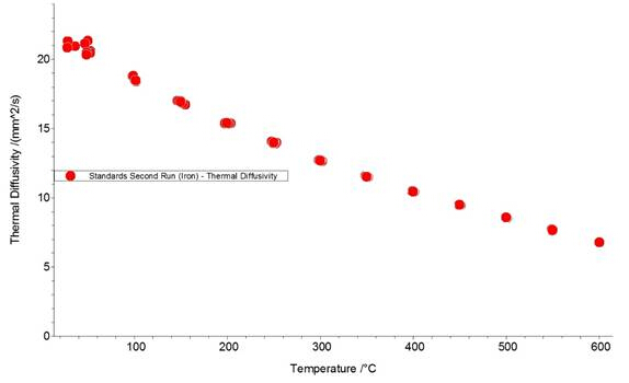
Figure 3: Thermal diffusivity (α) vs temperature plot for an iron standard disk, run in the LFA 457. Each red circle represents one laser pulse.

The laser flash method is a widely used technique for determination of thermal diffusivity which consists of radiating one side of a sample with thermal energy (from a laser source) and placing an IR detector on the other side to pick up the pulse. The wide range in temperature of different models enables measurement on various types of samples. The LFA requires relatively small samples. Other tools that measure thermal conductivity directly, rather than thermal diffusivity, include the Guarded Hot Plate, Heat Flow Meter and others. The Guarded Hot Plate system can hold relatively large square samples (300mm x 300mm) and requires careful calibration in order to calculate thermal flux necessary for thermal conductivity calculation. Neither of these tools can measure thermal diffusivity to high temperatures and typically operate below 250^oC.

Thermal diffusivity is an important property that needs to be known when choosing the appropriate material for any applications involving heat flow or that are sensitive to heat fluctuations. For example, thermal conductivity, aong with diffusivity, also play an important role in insulation. When selecting a material to use for insulation, it is important to be able to measure and compare the thermal properties of different materials. These thermal properties are even more critical in aerospace. Thermal protection tiles play an important role in a spacecraft's successful atmospheric re-entry. When entering the atmosphere, a spacecraft is exposed to extremely high temperatures and would melt, oxidize, or burn without a protective layer. Thermal protection tiles are typically made of pure silica glass fibers with tiny air-filled pores. These two components have low thermal conductivity and therefore minimize heat flux across the tiles. The thermal conductivity of materials with a high porosity () can be calculated with the following Maxwell's relation :
    (Equation 2)